Fluid flow in hydrocyclones optimized through multi-objective genetic algorithms

Abstract

Transient swirl flow fields that exist in the hydrocyclone separators have been simulated using the CFD software FLUENT™. The outputs are treated in a multi-objective fashion using tailor-made evolutionary computing softwares developed in-house. The recently proposed ‘new multi-objective genetic algorithm’ developed at this research group is utilized for this purpose along with a multi-objective immune system algorithm. Using the simulated flow fields, attempts are made to simultaneously optimize two conflicting criteria: (i) the volume of the LZV (locus of zero vertical velocity) envelope that governs the extent of classification towards the overflow region and (ii) the overall pressure drop that drives the classification process towards the underflow. The resulting Pareto frontiers are computed and analysed.

Keywords:

• flow configuration
• hydrocyclone
• NMGA
• Pareto frontiers
• CFD
• genetic algorithms
• multi-objective optimization

1. Introduction

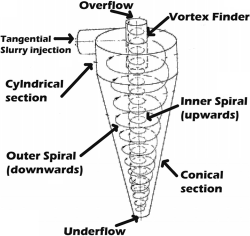
Hydrocyclones are ubiquitous in mineral processing industries 1. They are also being commonly used for raw material preparation in many integrated steel plants. The hydrocyclones ingeniously utilize some of the fundamental features of swirl flow 2. The basic configuration includes a cylindrical region above an inverted cone. The feed, usually slurry, is injected tangentially at the top and traditionally the flow is visualized as a conglomerate of two concentric spirals: the outer one carries the denser particles to the underflow, while through a vortex finder at the upper region of the device the lighter particles reach the overflow (Figure 1).

Figure 1. Schematic diagram of a hydrocyclone showing the swirl.

The flow configurations in the hydrocyclone and its related devices have become the topic of a number of earlier works 3 and a limited number of studies also exist 4 where the nature inspired evolutionary algorithms 5,6 have been utilized to study them. An enormous scope of developing some basic understanding of the fluid motion in a hydrocyclone by using a flow solver in tandem with an evolutionary optimizer capable of handling more than one conflicting criteria still exists. In this study, we have attempted to achieve that by using two evolutionary algorithms: (i) a multi-objective immune system algorithm 7 and (ii) a new multi-objective genetic algorithm 8 developed earlier in this research group. We begin with a brief description of each.

2. Multi-objective immune system algorithm

The multi-objective immune system algorithm (MISA) used in this study is a slightly adapted version of an earlier strategy proposed by Coello Coello and Cortés 7. When some harmful antigens invade our body, it triggers off antibodies through the immune system to combat them. Mimicking these phenomena in quite a naïve way, the strategy proposed by Coello Coello and Cortés 7, splits the usual binary genetic algorithms population into antigens and antibodies. This classification is based upon Pareto dominance as well as the feasibility of the solutions, the basic concepts of which are readily available in the literature 5,6. A strength parameter is also assigned to each antigen: the strongest ones being those leading to feasible and non-dominated solutions. The lowest strength on the other hand is assigned to the antigens that are feasible but dominated by others, and an intermediate strength is prescribed for those, which are non-dominated but infeasible. In nature, a particular antibody remains specific to some particular antigen: for example, the antibody that protects us from cold virus may not be of any use if we are infected by chicken pox. In the present algorithm, each antigen is made specific to a particular antibody by randomly pairing the members of the respective sub-populations. A fitness value is now assigned to each antibody based upon its extent of matching with its associated antigen and the strength of the antigen itself. A number of better antibodies are now selected from the pool and are cloned by making a prescribed number of copies for each. The clones are now mutated mimicking the phenomenon of hypermutation in the natural system: the more dissimilar the clone is from its prescribed antigen, higher its mutation rate. Once the mutation stops, an enhanced population is created by mixing the mutated clones with the original antibodies, from which the non-dominated and feasible members are taken out to create the next generation, keeping the population size unaltered. Like the original procedure 7 the strongest antigens at the onset of each generation are kept in a repertoire called the secondary memory. The entrants there are like the memory cells in the natural systems, which tells the body how it built its defence against a certain antigens when the same one infects it once again. In the algorithm of Coello Coello and Cortés 7, the information contained in this memory cell repertoire had actually remained underutilized. In the current variant of this algorithm, some random memory cell members are periodically migrated to the antibody population as an attempt to introduce some elitism in the system. Unlike the conventional genetic algorithms, the whole procedure was kept mutation driven and no crossover operator was introduced since it is not relevant for the biological immune systems. This procedure was repeated for a predefined number of generations deemed adequate to attain convergence.

3. A new multi-objective genetic algorithm

This algorithm was developed recently in this research group 8 and was used in this investigation along with the artificial immune strategy described above. During its development stage, new multi-objective genetic algorithm (NMGA) was elaborately tested on the ZDT test functions 6 and was also applied to a real-life steel plant problem.

In this algorithm, a traditional genetic algorithm population is mapped on to a discretized functional space ‘f ’ where each member is assigned to a particular grid location ‘g’. For I objective functions, the indices of the grid can be designated through an integer coordinate system , related to the corresponding objective functions as: (1) where the subscripts indicate the lower and upper bounds of the function and n denote the total number of grids that the user needs to specify. A particular grid location, in principle, can be inhabited by more than one member of the population, provided they have got identical indices.

3.1. Recombination process in a flexible Moore neighbourhood

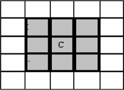
Once the entire population is mapped on to the functional space, a neighbourhood 9 is assigned to each of them. What we have used here is esentially a Moore neighbourhood 9, shown schematically in Figure 2 with some flexibilty added to its conventional form. In the present context, genetic recombination entails crossing over the central member C with a random partner from the shaded region. In case no such partners are found, for a neighbourhood being occupied only by C, it is further expanded by adding more layers of grids, but maintaining the required symmetry, until at least one additional individual is located. The children are also appropriately placed in the functional space, and a pruning of the population is undertaken, as elaborated below.

Figure 2. The concept of Moore neighbourhood.

3.2. Ranking the population

Once the genetic recombination and mutation is finished, all the dominated individuals in the neighbourhood are deleted. The resulting population is then ranked, where one has the option of following either the Goldberg or the Fonseca approach 5,6. In the former, the non-dominated members of the population are taken out of the population as rank one. The truncated population is again checked for non-dominance and another set of individuals is once again removed and placed as rank two members, and the procedure continues. In the Fonseca strategy, the entire population is checked for dominance and the ranks to the individuals are assigned using the formula: (2) where R_i is the rank of the individual i, and N_d is the number of individuals that dominate it.

The Fonseca approach involves a lesser computational burden and was therefore preferred in this study. The rank information allows further downsizing of the population and the procedure is elaborated below.

3.3. The procedure for rank-based population sizing

New multi-objective genetic algorithm allows both the parents and their children to be present in the population; the population size often tends to grow unmanageably large because of that. Even after removing the dominated solutions in the neighbourhood this problem tends to persist. Based upon the rank information, the population is therefore trimmed further. The main idea behind the population sizing procedure adopted here is to ensure that the representatives of every rank are present in the final population of size S and the extent of representation remains largest for rank one and becomes progressively lower as the rank index increases. To achieve this, initially all the individuals are ranked using the Fonseca strategy, and the value of N_R, the permitted number of individuals of rank R in the final set, is computed by the function: (3) where the constant N_O is calculated using the value of S. Since no upper limit is imposed on the values of the ranks, in principle, we can take the maximum rank as infinity while the lowest, by definition, is unity, which constitute the Pareto front. Thus, the total set S should be equal to the sum of the permitted number of individuals of all ranks, such that (4) Substituting the values of N₁,N₂,N₃,…,N_∞ into Equation (4), the final equation becomes: (5) Summing up the infinite series in geometric progression, the value of N_O is calculated as: (6) However, owing to this procedure the value of N_R will become <1 for the ranks above ln(N_O), implying that these individuals will not be represented in the population, even if some slots might still be available. In order to rectify this problem, a slightly modified form of the original function was taken such that: (7) The next generation started with the population adjusted in this fashion and the procedure continued for a prescribed number of generations.

4. Multi-objective modelling of the swirl flow field

A rigorous description of the swirl flow field would entail a closed form solution of the 3D Navier–Stokes equations in their transient form. The flow equations and the pertinent boundary and initial conditions could be described as follows.

Volume of fluid model: the volume of fluid method for two fluids/phases is based on the assumption that the fluids are not interpenetrating. The properties appearing in the transport equations are determined by the volume fraction α_i of the component phases in each control volume. The corresponding equations for a two phase system is shown as where ρ is the effective density of the system and the volume fraction of the second component is being tracked.

All other properties (e.g. viscosity) are computed in the same manner. A single set of Navier–Stokes equations is solved where the velocity field is shared among the phases, through the effective properties definitions.

Equation of continuity: (8) Conservation of Momentum Equations: (9) Swirl number: (10) where is the hydraulic radius and ω in the swirl number formula represents the angular velocity of fluid particles. The swirl number ‘S’ represents the ratio of the axial flux of the swirl momentum to the axial flux of the axial momentum times the hydraulic radius. Hence, the area element is taken on the surface perpendicular to the axial direction.

For low swirl, i.e. S < 0.5, RNG k − ε model is recommended and for high swirl, i.e. , Reynolds stress model (RSM) is recommended.

In case of the turbulence model, a single set of transport equations is solved and the Reynolds stresses are shared by the phases throughout the field.

Reynolds stress model: (11) (12) The RSM models were sucessfully used earlier for the turbulence closure in the cyclonic devices 3. In recent times, the application of large eddy simulation procedure (LES) has also been gaining ground 10. The ubiquitous k − ϵ turbulence model however tends to become less reliable in case of hydrocyclones, since in a situation of high swirl, contrary to the requirement of this model, the structure of turbulence tends to become predominately anisotropic 3.

No slip conditions were applied to all the inside wall surfaces of the hydrocyclone body, including the inside surfaces of the inlet and the vortex finder. Continuity of shear stress was implemented at the interface between the air core and the swirling slurry. Initially the hydrocyclone was assumed to be completely filled with air, i.e. the initial air fraction inside the hydrocyclone was assumed to be unity.

4.1. The task of optimization

The axial fluid flow inside the hydrocyclone is characterized by a flow reversal 3, causing the build up of an inner upward spiral mentioned before. For many control volumes, as they move down the device, the vertical velocity component changes its direction, from initially downwards to upward at some point. This necessitates the axial velocity to become zero at a particular location. The locus of the zero vertical velocity points (LZV) traced by all such control volumes constitutes an envelope and the volume enclosed by it directly affects amount of lighter materials reporting at the overflow through the vortex finder located at the upper region of this classifier. The coarser material reporting at the underflow is predominately conveyed by the downward moving outer spiral, and the amount of material reaching there is directly dependent on the axial pressure drop that exists in the hydrocyclone. Keeping these in mind, here we have attempted to simultaneously optimize more than one criteria at a time, thus in some cases, leading to a situation where instead of a unique single solution, a family of fully non-dominated solutions 5,6, or in other words, the Pareto frontier would represent the best possible compromises in the objective space, and in turn would constitute the optima. The three scenarios that we have examined are as follows:

•	Maximize both pressure drop and the volume contained in the LZV envelope (referred later as the max–max problem).
•	Maximize the volume contained in the LZV envelope and minimize the pressure drop (referred later as the max–min problem).
•	Minimize the volume contained in the LZV envelope and maximize the pressure drop and (referred later as the min–max problem).

The first instance leads to a conflicting situation where the particle collection both at the overflow and the underflow are simultaneously being maximized and the best possible compromises are expected to lead to a Pareto frontier. The second situation renders the flow biased towards the overflow, and the converse remains true for the third case.

Both the pressure drop and the volume contained by the LZV envelope could be determined only through the flow solutions. In the evolutionary strategies mentioned here, one needs to know them for each and every population member at any generation. In situ computation of these two objectives during the optimization runs required simultaneous time exhaustive CFD simulations, and that too for a large number of population members, which was not feasible due to various computational constraints. To circumvent this inconvenience, flow simulations were separately conducted with a substantial variation in the decision variable space and the computed values of pressure drop and the LZV volume were passed on to the evolutionary algorithms as two fitted polynomials. The formulas for both f₁(v) and f₂(v) were determined by keeping the density constant at 1400 kg m⁻³, and the formula for both f₁(ρ) and f₂(ρ) was determined by keeping v = 2.65 m s⁻¹. All the above relations are the result of curve-fitting after the separation of variables. In the combined function, shown below, the division by two was done according to the mean-square formulation. While there are many ways to combine the two functions, this particular relation was used because the independent functions were given equal weights. Particularly for the pressure drop in the hydrocyclones and related devices, experimental pressure drop values have often been correlated with the similar process variables in similar polynomial forms 3, and polynomial representation of the LZV envelope is in general agreement with the existing axial velocity correlations 3 as well. The basic equations associated with the optimization task of the objective functions f₁ and f₂ are summarized below. The velocity v and density ρ are the decision variables.

where

Total flow volume	=	= 0.000533 m3
Avg. inlet pressure	=	= 106483.26 Pa.

4.2. The computing task

The geometric details of the hydrocyclone simulated in this study are shown in Figure 3. Few additional design parameters are provided in Table 1. This represents a typical configuration used in the iron and steel industry. In addition, two other geometric configurations were also tried out on a few simulations, the details of which are provided in a subsequent section. The flow was computed using the commercial solver FLUENT™ (FLUENT 6.2, http://www.fluent.com) and the mesh generation was conducted with GAMBIT™ which is integrated with the CFD interface. A typical mesh is shown in Figure 4 and the various parameters associated with the flow simulation are provided in Table 2.

Figure 3. Schematic diagram of the simulated hydrocyclone with dimensions.

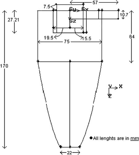
Figure 4. Mesh used in the hydrocyclone model.

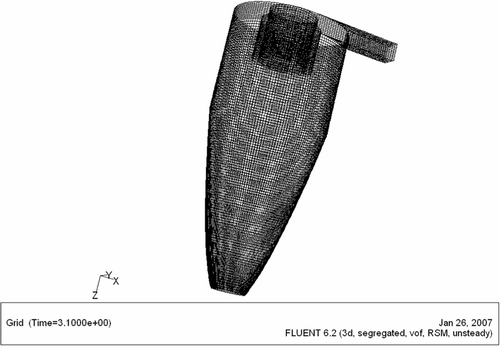
Table 1. Hydrocyclone design parameters.

Parameter	Type
Hydrocyclone design	Parabolic
Inlet type	Tangential inlet
Inlet cross section	Rectangular
No. of inlets	1

Table 2. Fluid flow simulation parameters.

Parameter	Type or value
Solver	3D Segregated (Unsteady)
Formulation	First-order implicit
Multiphase model	Volume of fluid
No. of Phases	2
Turbulence model	Reynolds stress model
Inlet slurry velocity	4–4.5 m s^−1
Slurry density	1200–2000 kg m^−3
Operating pressure	101,325 Pa

The codes for both evolutionary optimization algorithms were developed in-house and tested thoroughly on the ZDT test functions 6 before actually applying them to the present problem. The various parameters required for the evolutionary computation are summarized in Table 3.

Table 3. Genetic algorithm parameters.

Parameter	Value or Type
NMGA
Population size	100
Grid size	700 × 700
No. of generations	100
Crossover	Simulated binary 6
Distribution index	3
Mutation	Self adaptive
Mutation probability	1
MISA
Population size	100
Bit length	16
No. of fittest antibodies to be cloned	40
No. of clones of each antibody	10
No. of generations	1000–10,000
Mutation rate	(Z - matching between antigen–antibody pair)

5. Results and discussions

The transient flow solutions have allowed us to visualize the air core that forms along the hydrocyclone axis. Out of the numerous flow simulations that were carried out in this research, some representative results are shown in Figures 5–7.

Figure 5. Axial velocity vectors for ρ = 1400 kg m⁻³ and inlet slurry average speed v = 2.65 m s⁻¹ on the y = 0 plane.

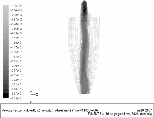
Figure 6. LZV for ρ = 1400 kg m⁻³ and inlet slurry average speed v = 2.65 m s⁻¹ on the y = 0 plane.

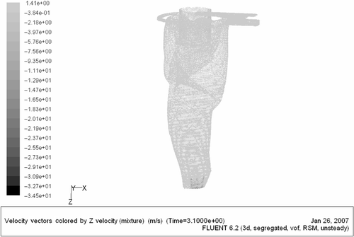
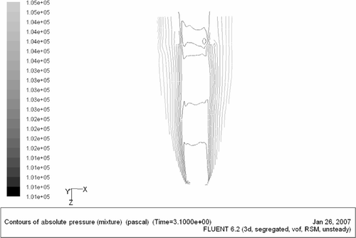
Figure 7. Contours of absolute pressure ρ = 1400 kg m⁻³ and inlet slurry average speed v = 2.65 m s⁻¹ on the y = 0 plane.

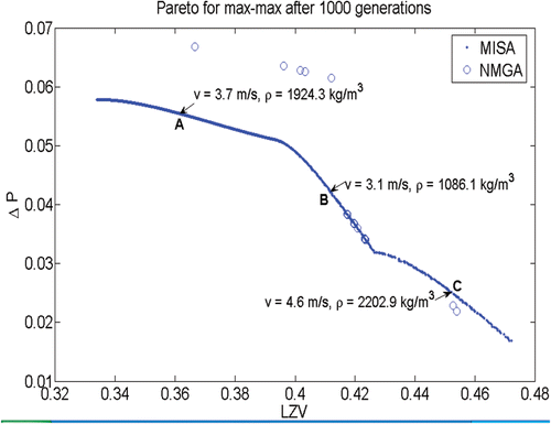
Several researchers have elaborately studied the basic features of swirl flow in this device earlier as discussed in 3. However, the major emphasis of this work was to come up with the flow fields optimized in a multi-objective fashion. The Pareto frontiers obtained for the three bi-criteria problems considered here are presented in Figures 8–10.

Figure 8. Pareto frontiers obtained for the max-max problems using NMGA and MISA. Typical decision variables are also shown.

5.1. The nature of the Pareto frontiers

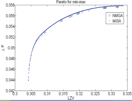
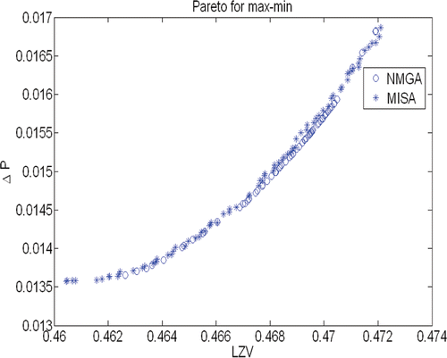
Understandably enough, the parameters LZV and ΔP are in direct conflict with each other as shown by the results of the max–max problem presented in Figure 8. An increase in one is inevitably associated with a decrease in the other. In other words, any attempt to bias the classification either towards the overflow needs to be compensated at the underflow and vice versa. The Pareto frontier depicts the best possible tradeoffs in this situation. In the remaining two cases, the ΔP and LZV are not at conflict with each other. However, a comparison of Figures 9 and 10 would reveal that in the function space the correlations between the objectives are different in case of max–min and min–max problems. In case of min–max problem, which is aimed at biasing the flow more towards the underflow, any attempt to do the same would be countered by a sharp response in the overflow side owing to the stiff slope of the frontier, particularly for the lower values of ΔP and LZV, as shown in Figure 9. Biasing the flow more towards the overflow side on the other hand can be done with a lesser disturbance of the velocity configurations at the underflow side, as suggested by rather gentle increase of the LZV with ΔP in the computed frontier of the max–min problem shown in Figure 10.

Figure 9. Pareto frontiers obtained for the min-max problem using NMGA and MISA.

5.2. Flow configurations of the optimal solutions

We would expect the flow profiles to vary from one end of the Pareto frontier to other. To ascertain this, flow simulations have been conducted for the three different Pareto optimal solutions A, B and C marked in Figure 8.

Figure 10. Pareto frontiers obtained for the max-min problem using NMGA and MISA.

Figures 11–13 show the static pressure contours for the three Pareto optimal solutions taken in the meridional y = 0 plane. The pressure in the air core is below atmospheric pressure as expected. There is also an axially downward pressure drop, the magnitude of which is comparable for all the three optimal solutions. However, for the Pareto optimal solution C the pressure contours are very well formed, which can be attributed to the fact that the solution C was allowed to converge more (lower magnitude of residuals) than the other two optimal solutions.

Figure 11. Contours of static pressure for optimal solution A.

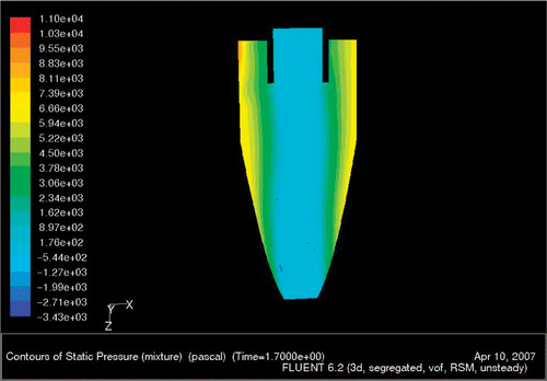
Figure 12. Contours of static pressure for optimal solution B.

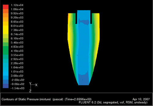
Figure 13. Contours of static pressure for optimal solution C.

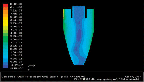
Figure 14. Axial velocity vectors for optimal solution A (right) and the optimal solution B (left).

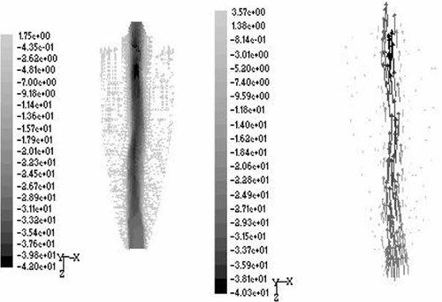
Figure 15. Variation of axial velocity with the radius on either side of the axis at Z = 100 mm.

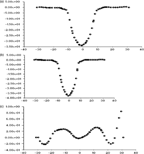
Figure 16. Variation of radial velocity with the radius on either side of the axis at Z = 100 mm.

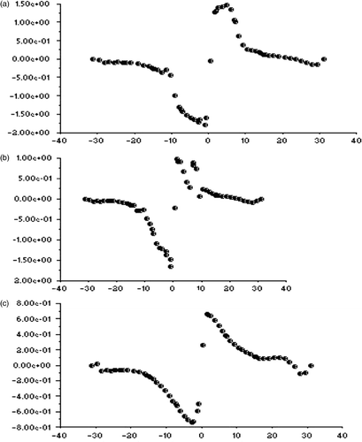
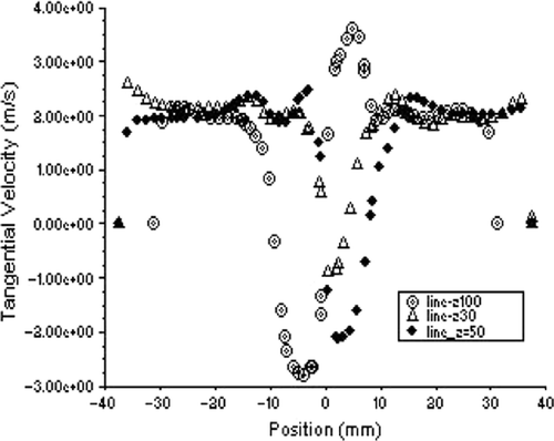
Figure 17. Variation of tangential velocity with the radius on either side of the axis at Z = 100 mm.

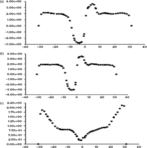
Figure 18. Variation of axial velocity with the radius on either side of the axis at different Z, for solution A.

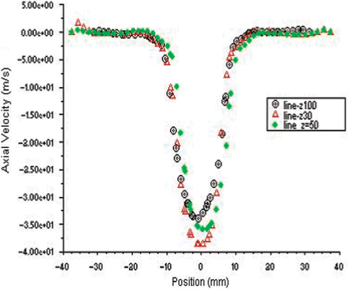
Figure 19. Variation of axial velocity with the radius on either side of the axis at different Z, for solution A in the regions of axial flow reversal.

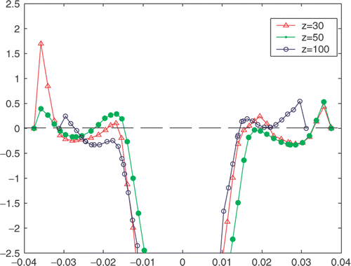
Figure 20. Variation of radial velocity with the radius on either side of the axis at different Z, for optimal solution A.

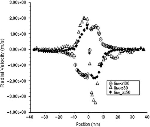
Figure 21. Variation of tangential velocity with the radius on either side of the axis at different Z, for optimal solution A.

Figure 14 shows the velocity vectors of the optimal solutions A and B in y = 0 plane. A dynamic air core is formed which can be attributed to a relatively high-axial velocity in that region compared to that in the slurry.

Figures 15–17 show the variation of axial radial and tangential velocities with the radius on either side of the axis of the hydrocyclone for the optimal solutions A, B and C, marked correspondingly as (a), (b) and (c) in the figures. Axially downward direction of the hydrocyclone is taken as the positive z direction in all the cases. It appears that the axial and radial velocities are almost axi-symmetric, while the tangential velocity is not. This is expected as both the axial and radial velocities have a weak dependence on the direction of swirl, or in other words, the angular gradient of the axial velocity ∂v_z/∂θ and also that of the radial velocity ∂v_r/∂θ are negligible. Consequently, the absence of axi-symmetry in the flow due to its swirl nature is not manifested in the axial and radial velocity profiles. This is also supported by the fact that ∂v_z/∂θ and ∂v_r/∂θ have got no contributions in the continuity of the mass flow of the swirl which could be stated as The radial variation pattern of the axial and radial velocities, especially the axial velocity, does not change with z, as shown in Figures 18–21. However, the magnitude of maximum radial velocity decreases axially downward, which is due to the decreasing radius of the conical section. There is an interesting observation in case of the radial variation of the radial velocity shown in Figure 20. The direction of radial velocity is inward in the upper cylindrical portion of the hydrocyclone and outward in the lower conical portion. This can be attributed to the change in the other velocity gradients as exhibited by the continuity equation. The difference between the maximum upward axial velocity at z = 30 mm and z = 100 mm can be attributed to the continuity of mass flow, considering the significantly lower radius of cross section at z = 100 mm. This exhibits the formation of the concave LZV contour, where the magnitude of axial velocity reversal decreases axially downwards. On the other hand, a close examination of Figure 19 reveals that the inner point of inflection in the axial velocity remains almost at the same radial location for different z values, indicating the consistency in the diameter of the air core along the axis of the hydrocyclone. However, as shown in Figure 21, the tangential velocity undergoes a change in its radial variation pattern with changing z. This exhibits the lack of axi-symmetry in the flow, which is also manifested by the shift of eye of the swirl with increasing z values measured axially downward.

5.3. The effect of hydrocyclone geometry

Although most of the simulations in this study, and all the results presented so far, have been conducted for the hydrocyclone design shown in Figure 3, it is also deemed appropriate to explore the impact of a geometry variation of the hydrocyclone. Two more geometries shown in Figure 22, which are also relevant for the steel industries, are thus subjected to some additional simulations. Further details of those designs are provided in Table 4.

Figure 22. Two additional geometries of the hydrocyclone.

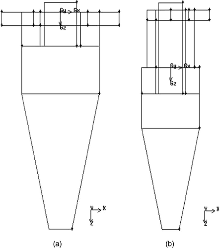
Table 4. Hydrocyclone design parameters.

Geometry	Parameter	Type
a	Hydrocyclone design	Conical
	Inlet type	Tangential
	Inlet cross section	Rectangular
	No. of inlets	2
b	Hydrocyclone design	Conical
	Inlet type	Extended
	Inlet cross section	Rectangular
	No. of inlets	1

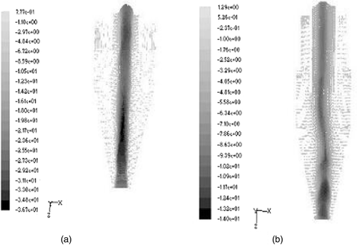
The velocity profiles exhibited by the vector plots of the corresponding axial velocities are shown in Figure 23. The hydrocyclone (a) has a relatively symmetrical velocity profile which may be attributed to the presence of two tangential inlets located diametrically opposite to each other. The hydrocyclone (b) shows a very stable air core in the upper portion, due to the presence of an extended part. Geometry therefore plays a significant role which needs to be accounted for while analysing the flow structure in a hydrocyclone.

Figure 23. Axial velocity vectors of hydrocyclone (a) and (b).

5.4. Performance of the two algorithms

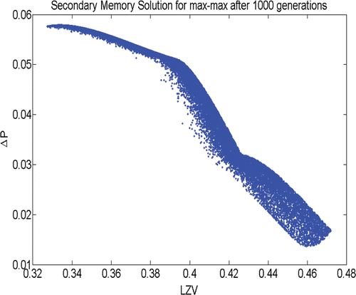
In case of the max–min and min–max problems (Figures 9 and 10) both NMGA and the immune algorithm MISA have shown very similar results. However, in case of the max–max problem (Figure 8) the results have shown some difference. In few instances, particularly in the region ‘A’ NMGA has converged to some better solutions, the solutions remained basically similar in ‘B’, the mid-range of the frontier, while in region C the NMGA solutions tend to become a bit inferior. Although NMGA has provided better quality solutions in few cases, the overall diversity of the solutions obtained through MISA are generally better, as they are more evenly spread in the functional space, covering the entire range of the Pareto frontier. This ability of MISA partly comes through its elitist strategy performed through the periodic usage of its secondary memory which indeed acts as an excellent repertoire of the promising solutions at all ranges, as shown in Figure 24. The efficacy of MISA could be further improved with more efficient handling of the information stored in the secondary memory.

Figure 24. Secondary memory repertoire for the max-max problem in MISA.

6. Concluding remarks

For any commercial hydrocyclones adjusting the process variables for a proper cutoff size is a challenging task, where the procedures shown in this article can come to the aid of the decision maker. Coupling a CFD procedure with a multi-criteria evolutionary approach is emerging fast in many disciplines 11, 12. This successful application to the hydrocyclones is aimed at moving it a step further removing the obsolescence of some earlier work 13, 14 that was based upon some simplistic assumptions and were devoid of any attempts of optimizing the flow field.

Acknowledgements

The authors are thankful to TATA Steel for funding this research, to Prof. G.S. Dulikravich for his generous invitation and financial support during the IPDO 2007 conference and to B. Siva Kumar and V. Satish Babu for their preliminary work on NMGA.

References

- Svarovsky, L, 1984. Hydrocyclones. New York: Tecnomic Publishing Co.; 1984.
- Soo, SL, 1989. Particulate and Continuum: Multiphase Fluid Dynamics. New York: Hemisphere; 1989.
- Chakraborti, N, and Miller, JD, 1992. Fluid flow in hydrocyclones: a critical review, Mineral Process. Extr. Met. Rev. 11 (1992), pp. 211–244.
- Karr, CL, Stanley, DA, and McWhorter, B, 2000. Optimization of hydrocyclone operation using a geno-fuzzy algorithm, Comp. Methods Applied Mech. Eng. 186 (2000), pp. 517–530.
- Coello, CA, et al., 2002. Evolutionary Algorithms for Solving Multi-Objective Problems. New York: Kluwer; 2002.
- Deb, K, 2001. Multi-objective Optimization using Evolutionary Algorithms. Chichester: John-Wiley; 2001.
- Coello Coello, CA, and Cortés, NC, 2002. "An approach to solve multiobjective optimization problems based on an artificial immune system". In: Timmis, J, and Bentley, PJ, eds. First International Conference on Artificial Immune Systems (ICARIS'2002). Canterbury: University of Kent; 2002. pp. 212–221.
- Chakraborti, N, et al., 2008. A new multi-objective genetic algorithm applied to hot-rolling process, App. Math. Modelling 32 (2008), pp. 1781–1789.
- Pettersson, F, Chakraborti, N, and Saxén, H, 2007. A genetic algorithms based multi-objective neural net applied to noisy blast furnace data, App. Soft Comput. 7 (2007), pp. 387–397.
- Delgadillo, JA, and Rajamani, RK, 2005. A comparative study of three turbulence-closure models for the hydrocyclone problem, Int. J. Mineral Process 77 (2005), pp. 217–230.
- Kumar, A, et al., 2005. Gas injection in steelmaking vessels: coupling a fluid dynamic analysis with a genetic algorithms based Pareto-optimality, Mat. Manuf. Processes 20 (2005), pp. 363–379.
- Colaço, MJ, and Dulikravich, GS, 2007. Solidification of double-diffusive flows using thermo-magneto-hydrodynamics and optimization, Mat. Manuf. Proces. 22 (2007), p. 594.
- Das, A, et al., 1993. Fluid motion in air-sparged hydrocyclone – single-phase measurements and calculations of tangential velocity of swirl flow in a right-vertical cylinder, Scand. J. Metallurgy 22 (1993), p. 254.
- Narasimha, M, Sripriya, R, and Banerjee, PK, 2005. CFD modelling of hydrocyclone-prediction of cut size, Int. J. Min. Proces. 75 (2005), p. 53.