Global optimization of thermal conductivity using stochastic algorithms

Abstract

In this article, the performance of a self-organizing migration algorithm (SOMA), a new stochastic optimization algorithm, has been compared with a genetic algorithm with floating-point representation (GAF) and differential evolution (DE) for an engineering application. This application is the estimation of the apparent thermal conductivity of foods at freezing temperature using an inverse method. Assuming two piecewise functions for apparent thermal conductivity in function of the temperature data, the heat diffusion equation was solved to estimate the unknown variables of inverse problem. The thermal conductivity is continuously adjusted by three approaches of stochastic optimization algorithms, used to minimize a performance criterion based on error information for the inverse problem. The variables that provide the best fitness between the experimental and predicted time-temperature curves at centre of the food under freezing conditions were obtained. Moreover, a statistical analysis showed the agreement between reported and estimated curves. In this application domain, the SOMA and DE approaches outperform the GAF.

Keywords:

• inverse problem
• thermal conductivity
• optimization
• genetic algorithm
• differential evolution
• self-organizing migration algorithm
• food

Nomenclature

c	=	random value in GAF
cp	=	specific heat (J kg−1°C−1)
CR	=	crossover or recombination rate in DE
DE	=	differential evolution
f	=	objective function
fm	=	mutation factor in DE
g	=	parameter in SOMA
GAF	=	genetic algorithm with floating-point representation
h	=	heat transfer coefficient (W m−2°C−1)
H	=	volumetric specific enthalpy (J m−3)
IHTP	=	inverse heat transfer problem
k	=	thermal conductivity (W m−1°C−1)
L	=	half length in x direction (m)
	=	difference between leader and start position of individual in SOMA
N	=	size population (individuals); number of samples
N (0,1)	=	random number with Gaussian distribution, zero mean and variance one
PRT	=	parameter in range [0, 1] in SOMA
	=	perturbation vector in SOMA
rnd	=	random number generation
r	=	vector candidate solution in SOMA
R2	=	Pearson multiple correlation coefficient index
SOMA	=	self-organizing migration algorithm
t	=	coordinate in freezing time (s)
T	=	theoretical temperature (°C)
τ	=	experimental temperature (°C)
u	=	trial vector in DE
x	=	vector solution
z	=	mutant vector in DE

Greek symbols

β	=	step length used in BFGS evaluated by Armijo or index for indicates vectors in DE
δ	=	recombination mechanism in DE
ϵ	=	tolerance value
ρ	=	density (kg m−3)
φ	=	index that indicates the method for selecting of the parent chromosome in DE
Δt	=	temporal mesh step (s)
Δx	=	spatial mesh step (m)

Subscripts

i	=	index represents mesh interval or individuals for optimization algorithms
j	=	index represents time interval or dimensions problem space
l	=	leader in SOMA
max	=	maximum
n	=	dimension of the vector solution
npop	=	size population
r1, r2, r3	=	integers used in DE
0	=	initial
∞	=	ambient

Superscripts

ct	=	generations counter
L	=	lower boundary
tt	=	time indicator
U	=	upper boundary
*	=	reference which corresponds to null enthalpy

1. Introduction

The development of the inverse heat transfer problem (IHTP) has progressed rapidly with the help of new mathematical approaches and modern computational facilities. Recently, optimization methods were applied to solve the IHTP. The main idea in the optimization methods is to minimize (or maximize) one or more objective function(s) that is defined in such a way that the minimum (or maximum) corresponds to the best design configuration.

Unlike the conventional techniques, the resolution of the IHTP permits the determination of more than one thermo-physical property and the understanding of complex materials. Different optimization techniques, such as conjugate gradient and Levenberg–Marquardt methods were employed to estimate the thermo-physical properties in recent literature 1–7. Modern optimization methodologies are being used to solve inverse problems, particularly stochastic methods, which usually supply potential solutions, but the computational time required by stochastic methods generally exceeds that of deterministic optimization methods 8,9. Other optimization techniques based on computational intelligence approaches, such as genetic algorithms and artificial neural networks, were also used for the solution of IHTP 10–15.

More related to the present contribution are the following works. Sawaf et al. 3 presented an inverse analysis to estimate a linearly-dependent temperature of thermal conductivity and heat capacity of an orthotropic solid. In that case, the Levenberg–Marquardt iterative procedure was used to solve the inverse problem. Yang 4 estimated the temperature-dependent thermal conductivity and heat capacity, simultaneously, from two temperature responses measured at the system boundaries. Kim et al. 5 proposed an integration approach to estimate the temperature-dependent thermal conductivity and heat capacity, simultaneously, in a one-dimensional non-linear heat conduction medium. The thermal properties were assumed to vary the time linearly with respect to temperature, and then were modelled as linear mathematical functions of temperature with unknown coefficients obtained by Levenberg–Marquardt method.

Znaidia et al. 6 estimated the effective thermal conductivity, the effective volumetric heat capacity as well as the heat transfer coefficient between a porous medium and a hot wire by a numerical inverse analysis. An iterative procedure, based on minimizing a sum of squares function with the Levenberg–Marquardt method was used to solve an inverse problem. Borukhov et al. 7 considered the problem of functional identification of the non-linear thermal-conductivity coefficient. For numerical solution of inverse heat-conduction problem, Borukhov et al. 7 used an optimization method based on gradient information. Mendonça et al. 16 estimated the thermal conductivity and volumetric thermal capacity of apples through of the methodology based in the inverse problem of heat conduction solution. Mariani et al. 17 applied differential evolution (DE) algorithm for the estimation of apparent thermal diffusivity of bananas at different drying temperatures. Parameters of two functions, the first dependent of the moisture content and the second also dependent of the temperature were obtained by the inverse method.

According to our knowledge there are few works in literature that estimate the thermo-physical properties of foods during the freezing process, and no work in the literature was found combining inverse problems and self-organizing migration algorithms (SOMA) to estimate the thermal conductivity. There are some methods to measure the thermal conductivity proposed in the specialized literature, nevertheless, most of them need relatively complex instrumentation or experimental assembles and demand an expertise of the thermal phenomena.

In this work, the inverse problem is solved as an unconstrained optimization problem in which the multiple correlation index, R², is maximized, and the objective function, f, is minimized. Three optimization methods of evolutionary computation field including SOMA, genetic algorithm with floating-point representation (GAF) and DE are evaluated to solve an inverse problem of heat conduction. Stochastic optimization methods of evolutionary computation have yielded promising results for solving non-linear, non-differentiable and multi-modal optimization problems 18–23. The inverse problem considered here is relevant in food processing operations, such as the analysis of transient heat transfer during the drying, cooling or freezing of fruits and vegetables in continuous systems, which requires knowledge of the thermal properties of the products.

In this context, the goal of this study is to explore and analyse the performance of SOMA, a stochastic optimization algorithm recently proposed in literature, when compared with GAF and DE accurately estimating the time-varying thermal conductivity of the carrot purée in −38.5°C to the freezing temperature. The enthalpy formulation of the heat conduction process utilizes two dependent variables, enthalpy and temperature. Such formulation is used in this study, and the thermal conductivity is obtained via the inverse method. The estimation is based on transient temperature measurements taken by a thermocouple on the inner part of the carrot purée.

The remainder of this article is organized as follows. In Section 2, the stochastic optimization algorithms: GAF, DE and SOMA are described. In Section 3, the case study is presented, i.e. the mathematical formulation of the transient heat conduction problem, the experimental tests and optimization problem are presented. Numerical results based on simulated experimental data are presented and discussed in Section 4. In the same section, the performance of tested optimization algorithms is shown using statistics parameters. Lastly, Section 5 summarizes our conclusion.

2. Stochastic optimization algorithms

In recent years, a class of algorithms has been developed for stochastic optimization, i.e. for optimizing systems where the functional relationship between the independent input variables and objective function of a system is not known. Using stochastic optimization algorithms of evolutionary computation field such as genetic algorithm, evolution strategies, evolutionary programming and DE, a system is confronted with a random input vector and its response is measured. This response is then used by the algorithm to tune the input vector in such a way that the system produces the desired output or target value in an iterative process. These algorithms share a common conceptual base simulating the evolution of individual structures via selection and reproduction procedures. The basic idea is to maintain a population of candidate solutions that are evolved in generations in which only the best-suited–or fittest–individuals are likely to survive 18,19.

The stopping criterion for GAF, DE and SOMA should be that the fitness function is less than or equal to some tolerance, f(x) ≤ ξ, or that the maximum number of generations has been exceeded, ct_max. Three different algorithms were used in this work to obtain the apparent thermal conductivity using inverse method. The main principles of the algorithms are described below.

2.1. Genetic algorithm with floating-point representation

The GA is a search technique based on the concepts of natural selection and natural genetics, which combines an artificial survival of the fittest with genetic operators abstracted from nature. In the present work, the GAF consists of three genetic operators (selection, crossover and mutation). Discussion about GAF operators is presented in Michalewicz 24, Michalewicz et al. 25 and De Jong 26. The procedure of GAF is described in the next sections.

2.1.1. Generation of initial population

The generations’ counter, ct = 1, is initialized and a population for i = 1, …, n_pop of individuals with random values generated according to a uniform probability distribution in the n dimensional problem space is initialized. These initial individual values are chosen within user-defined bounds, , where is lower boundary constraints and is upper boundary constraints for j = 1, …, n, ∈ D = IRⁿ, and D is a convex set, where (1)

2.1.2. Evaluation of fitness

The individuals are evaluated based on their performances in terms of objective function value, i.e. each individual is evaluated according to a fitness function.

2.1.3. Selection

The reproduction operation is carried out by choosing individuals according to their relative fitness. In this operation, the selection mechanism called tournament is adopted. In selection by tournament, pr × n_pop individuals, where pr is the selection probability, with high-fitness are added into of the population, and pr × n_pop individuals with low-fitness are discarded from the population. The population still keeps the same size. Using this operator, high-fitness individuals are selected a greater number of times in proportion to their relative fitness. Reproduction operation alone cannot introduce any new (different) individuals into a population. The crossover and mutation operations are performed to generate new individuals.

2.1.4. Crossover

The crossover operator is believed to be the main search operator, and the purpose of this operator is two-fold. This binary operator is defined in this work as a linear combination of two vectors. If are to be crossed, the resulting offspring are . This operator uses a random value c ∈ [0, 1], as it always guarantees closeness. Thus, the crossover operation is carried out between two strings that are called parents. Two new strings are formed by the exchange of substrings between the parents, and they are called offspring. The offspring produced may or may not be more fit than the parents, depending on whether the crossing site falls in an appropriate place. Hence, every crossover might not be creating better solutions, but this does not cause a problem. If low-fitness offspring are created, they will be eliminated in the next reproduction operation, and hence will have a short life. On the other hand, if high-fitness offspring are produced, they are likely to increase in number in the next reproduction operation. Thus, this operation tends to enable the evolutionary process to move towards promising regions of the search space.

2.1.5. Mutation

The mutation operation is similar to the crossover operation and provides new individuals in the population by changing the value of the variable. The mutation operator is defined as follows. Each individual in the population can be subjected to mutation, with mutation rate in range [0, 1]. If an individual suffers mutation, the resulting individual is defined as (2) where N(0, 1) is a random number using a Gaussian distribution, with zero mean, and unitary variance. The mutation operation maintains the diversity of the population and prevents premature convergence to local optima.

2.1.6. Stopping criterion

The evolutionary procedure that has run reproduction, crossover and mutation operations once is called a generation. Set the generation number for ct = ct + 1. Sections 2.1.2–2.1.5 are repeated until a stopping criterion is satisfied.

2.2. Differential evolution

Differential evolution combines simple arithmetical operators with the classical operators of recombination, mutation and selection to evolve from a randomly generated population to a final solution. DE differs from conventional genetic algorithm in its use of perturbing vectors, which are the difference between two randomly chosen vectors. The DE algorithm was first introduced by Storn and Price 20, and was successfully applied in the optimization of some well-known non-linear, non-differentiable and non-convex functions by Storn 27.

The different variants of DE are classified using the following notation: DE/φ/β/δ, where φ indicates the method for selecting the parent chromosome that will form the base of the mutated vector, β indicates the number of difference vectors used to perturb the base chromosome and δ indicates the recombination mechanism used to create the offspring population. The bin acronym indicates that the recombination is controlled by a series of independent binomial experiments. The variant implemented was the DE/rnd/1/bin, which involved the following steps.

The user first chooses the parameters of population size, the boundary constraints of optimization variables, the mutation factor (or rate), f_m, the crossover rate, CR and the stopping criterion. The performance of a DE algorithm usually depends on three variables: n_pop, f_m and CR. The steps of adopted DE are described in the next sections.

2.2.1. Generation of initial population

The generations’ counter, ct = 1, is initialized and a population for i = 1, …, n_pop of individuals with random values generated according to a uniform probability distribution in the n-dimensional problem space, as used in GAF, is initialized, where (3)

2.2.2. Evaluation of fitness

Evaluate the fitness function of each individual in population.

2.2.3. Mutation

Mutation is an operation that adds a vector differential to a population vector of individuals according to the following equation: (4) where ct is the generation; stands for the position of the i-th individual of population of real-valued n-dimensional vectors; stands for the position of the i-th individual of a mutant vector; r₁, r₂ and r₃ are mutually different integers and also different from the running index, i, randomly selected with uniform distribution from the set {1,2,…,i − 1,i + 1,…,n_pop}, f_m > 0 is a real parameter called mutation factor, which controls the amplification of the difference between two individuals and is usually taken from the range [0.1, 1].

2.2.4. Recombination

Following the mutation operation, recombination is applied to the population. Recombination is employed to generate a trial vector by replacing certain parameters of the target vector with the corresponding parameters of a randomly generated donor vector.

For each vector, , an index i is randomly chosen using uniform distribution and a trial vector, , is generated with (5) where rnd_j is the j-th evaluation of a generation with uniform random number in the range [0, 1] and CR is a crossover (recombination) rate in the range [0, 1].

2.2.5. Selection

Selection is the procedure of producing better offspring. To decide whether or not the vector should be a member of the population comprising the next generation, it is compared with the corresponding vector, . Thus, if f denotes the objective function under minimization, then (6)

In this case, the objective function of each trial vector is compared with that of its parent target vector, . If the objective function, f, of the target vector is lower than that of the trial vector, the target is allowed to advance to the next generation. Otherwise, the target vector is replaced by trial vector in the next generation.

2.2.6. Stopping criterion

Set the generation number for ct = ct + 1 and go to Section 2.2.2 until a stopping criterion is met.

2.3. Self-organizing migrating algorithm

The SOMA is a optimization algorithm that is modelled on the social behaviour of co-operating individuals. It was chosen because it has proved that the algorithm has the ability to converge towards the global optimum 28.

2.3.1. Population

SOMA works with one population of candidate solutions in loops called migration loops. The population initialized is randomly distributed over the search space at the beginning of the search. In each loop, the population is evaluated and the solution with the highest fitness becomes the leader. Apart from the leader, in one migration loop, all individuals will traverse the input space in the direction of the leader. An individual will travel a certain distance (called the PathLength) towards the leader in k steps of defined length. If the PathLength is chosen to be greater than one, then the individual will overshoot the leader. This path is perturbed randomly. The initial population is generated in the same way as that in Equation (1) of GAF, which is needed to initialize the generations’ counter (in this algorithm called migrations), ct = 1.

2.3.2. Mutation

Mutation, the random perturbation of individuals, is an important operation for evolutionary strategies. It ensures diversity amongst the individuals and it also provides the mean store–lost information in a population. Mutation is different in SOMA compared with other evolutionary computation paradigms. SOMA uses a parameter called PRT to achieve perturbation. This parameter has the same effect for SOMA as mutation has for GAF. It is defined in the range [0, 1] and is used to create a perturbation vector, , as follows, (7)

The vector is created before an individual starts its journey over the search space. The vector defines the final movement of an active individual in search space.

2.3.3. Crossover

In SOMA, geometrical sequences of new positions are generated in the n-dimensional hyper-plane. They can be thought as a set of new individuals obtained by the special crossover operation. This crossover operation determines the behaviour of SOMA. The movement of an individual is thus given as follows: (8) where is the new candidate solution, is the original individual, is the difference between leader, l, and start position of individual, g ∈ [0, PathLength], and is the control vector for perturbation. Equation (8) can be rewritten as (9) where ct is the actual migration loop.

2.3.4. Stopping criterion

Set the migration (generation) number for ct = ct + 1 and go to Section 2.3.2 until a stopping criterion is met.

SOMA is controlled by a set of parameters. Some of these parameters are used to stop the search process when one of two criteria is fulfilled and the others are responsible for the quality of the results of the optimization process. The control parameters presented in Vascák 29 and Oplatková and Zelinka 30 are described as follow.

The PathLength ∈ [1.1, 3] defines how far an individual stops behind the leader (if one, stop at the leader's position, if two, stop behind the leader's position on the opposite side but at the same distance as at the starting point). If it is smaller than one, then the leader's position is not overshot, which carries the risk of premature convergence.

The step size ∈ [0.11, PathLength] defines the granularity with what the search space is sampled. In case of simple objective functions, it is possible to use a large step size in order to speed up the search process. If prior information about the objective function is not known, then the recommended value should be used. For greater diversity of the population, it is better if the distance between the start position of an individual and the leader is not a multiple of the step parameter. It means that a step size of 0.11 is better than a step size of 0.1, because the active individual will not reach the exact position of the leader.

The parameter ∈ [0, 1] determines whether an individual will travel directly towards the leader, or not. It is one of the most sensitive control parameters. The optimal value is near 0.1. When the value for is increased, the convergence speed of SOMA increases as well. In the case of low-dimensional functions and a great number of individuals, it is possible to set to 0.7–1.0. If vector equals 1, then the stochastic component of SOMA disappears and it performs only deterministic behaviour suitable for local search.

The n_pop, ∈ [10, up to the user] is the number of individuals in the population. The parameter migration, between 10 and up to the user, represents the maximum number of iterations. It is basically the same as generations for GAF or DE.

The MinDiv ∈ [arbitrary negative, up to the user] defines the largest allowed difference between the best and the worst individual from actual population. If the difference is too small, then the optimizing process is will stop. using small values is recommended, e.g. MinDiv = 1.

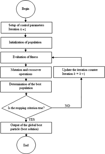
Figure 1 shows the basic pseudo-code for stochastic algorithms, including GAF, DE and SOMA, used in this study.

Figure 1. Pseudo-code for stochastic algorithms.

3. Problem formulation

Through Fourier law, a partial differential equation for both the phases is obtained making a balance of heat on a small region of the food, the form of this region depends on the system of coordinates adopted. Thus, the non-linear heat conduction problem, involving phase change, without internal heat generation, can be described over the spatial domain, Ω, in rectangular coordinates, by the heat equation 31 (10) where ρ (kg m⁻³) is the apparent density, c (J kg⁻¹°C⁻¹) is the apparent specific heat capacity, k (W m⁻¹°C⁻¹) is the apparent thermal conductivity, T (°C) is the temperature and t (s) is the time.

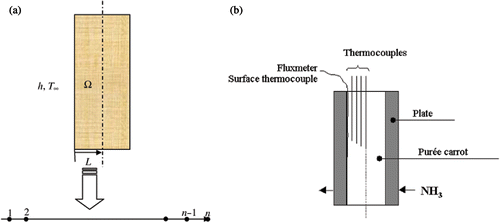
The present work considers one-dimensional geometry in rectangular coordinates, simulating a product slab, as shown in Figure 2(a). The initial condition associated to Equation (10) is (11) where T₀ (°C) is known temperature in initial time obtained through of experiment, t₀ (s) is initial time.

Figure 2. (a) Computational domain. (b) Diagram of the plate freezer with instrumentation.

In the food surface (x = 0), the convective condition is considered, (12) where T_∞ (°C) is the ambient temperature, h (W m⁻²°C⁻¹) is the surface heat transfer coefficient, L is the half length in x direction as shown in Figure 2(a).

The boundary condition used in the center of the product slab (x = L) was the classical zero flux, which is expressed by (13)

By performing a change in variables, the temperature-dependent density and apparent specific heat capacity in Equation (10) can be removed through of introduction of the volumetric specific enthalpy, H 32,33, , where T* (°C) is reference temperature which corresponds to the zero value of H.

With the introduction of the enthalpy, Equation (10) can be rewritten as 34 (14)

Due to the characteristics of the mathematical problem, the simpler finite difference technique 35,36 can be used rather than the finite element method or finite volume method for the solution of that partial differential equation. In this work, the explicit method is used. Using this numerical method, the heat balance for an element of unit cross section at the interior node i between levels t and t + Δt can written as (15)

Similar treatment of part element at node n yields the following difference equation, (16)

When the surface boundary condition specifies the surface temperature, heat balance of the part element at node 1 is acquired. With convective-type boundary condition, this heat balance is written and rearranged to yield the following equation: (17)

It is given credit that the precision of the numerical solution was not prejudiced by the adoption of the explicit method, as verified in the work of Cleland and Earle 37. When an explicit method is used it is necessary that the stability criterion should be satisfied, such criterion is satisfied in this study.

3.1. Experimental procedures

The plate freezer (Samifi Babcock, Germany) consists of vertical plates measuring 500 × 500 mm and distanced 90 mm from each other. Each plate is a part of the evaporator, inside which boiling ammonia is used as the coolant. The plates are distributed in a parallel arrangement forming compartments, where liquid or paste-like foods are fed by pumping. Figure 2(b) shows schematically a plate configuration.

It was observed that the thermal capacity of this plate does not influence the heat transfer in the purée. The equipment works in batch cycles, the product being charged hot and discharged when the centre reaches a desired temperature. Carrot purée (with 89.3% moisture content wet basis) was introduced in the equipment at 77°C and allowed to freeze until −15°C in the centre of the slab. The used cooling fluid in the interior of the plates is ammonia at −38.5°C. Four thermocouples (T-type, diameter 1.0 mm and 0.5 mm, accuracy ± 0.2°C) were inserted in the product, one in the centre and the three others, respectively, at 10, 20 and 30 mm from the centre, aligned. A surface thermocouple (Ref. 20117, type T, foil thickness 5 × 10⁻³ mm, surface area 63.0 mm², RdF Corp., USA) and a fluxmeter (27036-3, RdF Corp., USA) were adhered to the internal wall of a plate, in the interface with the product.

These instruments had allowed the measurement of the heat transfer coefficient between [400, 2000] W m⁻²°C⁻¹. The system composed by the instrumented carrot purée and its support was placed inside the freezing with ambient temperature T_∞ = −38.5°C. Each essay condition was repeated at least three times. At every time interval, the recorded heat flux, surface temperature and air temperature inside the freezing chamber were introduced in Equation (12) and the heat transfer coefficient was calculated straightforward. The average time for freezing was 120 min.

The resolution of the temperature measurement system was 0.1°C and the calibration in the range 100°C to −35°C resulted in a mean standard error of measurement of 0.7% in the scale extreme temperatures and an accuracy of ±0.2°C at 0°C.

3.2. Optimization formulation

Knowing the food geometry and physical properties, as the boundary and initial conditions, enables one to solve Equations (15–17), thus determining the transient temperature distribution in the food. This kind of problem is called a direct problem. If any of these magnitudes or a combination of them is unknown, but experimental data are available on the temperature measured inside and/or on the external surface of the food, one has an inverse problem that allows to determine the unknown magnitudes, provided those data contain sufficient information.

For the inverse problem of interest here, the apparent thermal conductivity is regarded as an unknown quantity. For the estimation of such parameters, we consider known transient temperature measurements τ_n (°C) taken at the centre node of the food. Thus, in this work it is desired to minimize the difference between experimental and predicted temperatures. The general form of the non-linear programming problem can be expressed as follows. Find to minimize (18) subject to boundary constraints (19) where T_n (°C) is the temperature of the carrot purée at node central, t (s) is the time indicator, calculated numerically by the explicit finite difference method and τ_n (°C) is the experimental temperature at thermocouple central, N is the number of samples and x_{i, j} is the vector of continuous variables.

In most of the techniques developed to solve inverse problems, the numerical model must be able to solve the direct problem with values arbitrated to the magnitudes to be determined. Since the procedures for the solution are usually iterative, the direct problem must be solved several times. Thus, it is desirable to have a precise method for the solution of the direct problem that requires a relatively short computational time. Numerical results are presented and discussed in the next section based on three stochastic algorithms.

4. Results and discussion

Analysing the temperature variation rate with the time in the centre of carrot purée, from the experimental data, it can be observed that the thermal conductivity must have a behaviour of decreasing accented next to reference temperature which corresponds to the zero value of H, and being practically constant in the next hours. Due to this fact, the use of two non-linear functions depending on temperature was proposed. The parameters were adjusted by inverse method using three stochastic approaches (see description in Section 2), so the number of parameters for adjust are five and three, using the Equations (20) and (21), respectively, (20) (21)

The proposed approach was analysed for the case in which five and three parameters for Equations (20) and (21), respectively, were treated as unknowns x_j for j = 1, …, 5, where the lower and upper boundaries constraints used for the vector were [1.6 5; 0.0001 1; −5 0.1; −1 1; 0 1] and [10⁻¹⁰ 0.05; −1 1; 0 1], respectively.

Each optimization approach was implemented in MATLAB (MathWorks). To illustrate the effectiveness of the optimization procedure, several simulations were performed. The parameters for all algorithms were set empirically, i.e. for each algorithm a number of tests with different parameter settings were carried out and the results were compared. The best settings were chosen, as shown in Table 1. Finding the best parameter settings is not an easy task, and can be complicated by the thermal conductivity drifting over time, i.e. its behaviour is not constant.

Table 1. Best parameter settings used in experiments.

GAF		DE		SOMA
npop	10	npop	10	npop	10
Selection rate	0.9	fm	0.4	MinDiv	0
Mutation rate	0.2	CR	0.8	PathLength	2.1
Crossover rate	0.8	Generations	100	Migrations	10
Generations	100			Step size	0.21
				PRT	0.5

In the tests, 10 independent runs were made for each optimization method involving 10 different initial trial solutions, n_pop. Numerical results can be seen in Figures 3–8 for all three algorithms. To quantify the effectiveness of different stochastic algorithms De Jong 26 devised two measures, one to gauge convergence and other to gauge ongoing performance. He called these measures off-line (convergence) and on-line (ongoing) performance, respectively. In an off-line application, many function evaluations can be simulated and the best alternative so far was saved and used after the achievement of some stopping criteria. An on-line application does not afford this luxury and function evaluations are achieved through real experimentation on line. In other words, the off-line performance is a running mean of the best performance values to a particular time. The on-line performance is a mean of all function evaluations up to and including the current trial. Both performances were used in this work.

Figure 3. Convergence for the best fitness of GAF using (a) Equation (20) and (b) Equation (21).

Figure 4. Convergence for the best fitness of DE using (a) Equation (20) and (b) Equation (21).

Figure 5. Convergence for the best fitness of SOMA using (a) Equation (20) and (b) Equation (21).

Figure 6. Convergence for the mean fitness of GAF using (a) Equation (20) and (b) Equation (21).

Figure 7. Convergence for the mean fitness of DE using (a) Equation (20) and (b) Equation (21).

Figure 8. Convergence for the mean fitness of SOMA using (a) Equation (20) and (b) Equation (21).

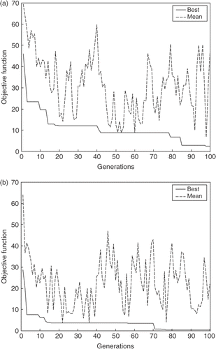
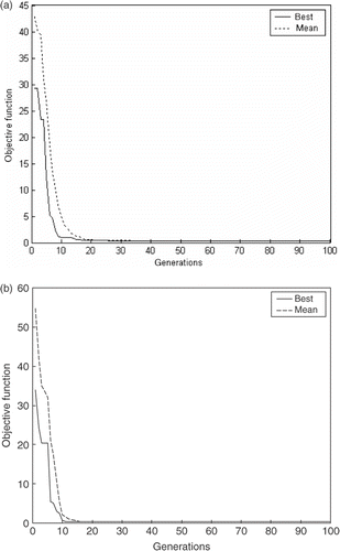
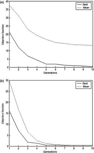
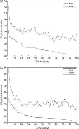
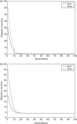
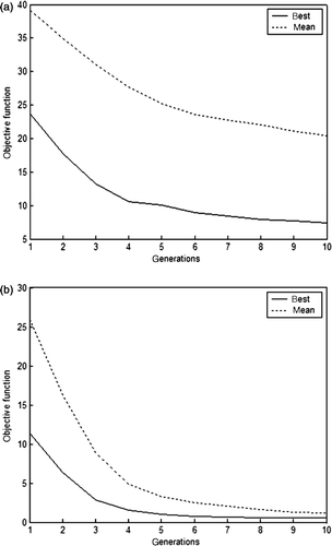
Figures 3–5 show the off-line performance, i.e. the best fitness of the population were stored for each generation in each run, since these values are made the mean and the best of each generation for GAF, DE and SOMA approaches are found, respectively. By comparing Figures 3–5 it is possible to identify that the GAF has the worst mean of 10 independent runs, while the DE and SOMA approaches show better performance than that the GAF.

Figures 6–8 show the on-line performance, i.e. in each generation the mean fitness of all population is calculated for all independent runs. Later on the best mean and the mean of mean in all 10 tests is found, for GAF, DE and SOMA, respectively. In Figure 6, the mean and best fitness values achieved for GAF are presented, where it can be seen that DE and SOMA presented better performance compared with GAF as shown in Figures 7 and 8, respectively, in this specific application. In Figures 7 and 8, note that the parameters obtained for Equation (21) showed the worse performance when compared with the parameters obtained for Equation (20).

The best fitness in the least squares sense between the experimental and numerical temperatures obtained by mathematical model is shown in Tables 2 and 3, for Equations (20) and (21), respectively. Deviations between experimental and simulated temperatures were calculated using the multiple correlation coefficient (Pearson coefficient), in successive trials as (22)

Table 2. Parameters of Equation (20).

Algorithms	x1	x2	x3	x4	x5	R^2	f
GAF	2.4431	0.0226	−3.1645	0.0051	0.5004	0.6912	2.4520
DE	2.4589	0.0487	−3.2515	−0.0024	0.7106	0.9932	0.3639
SOMA	2.4172	0.4628	−0.4970	−0.0011	0.6610	0.9894	0.4556

The R² value of 0.9–1.0 is considered sufficient for that apparent thermal conductivity obtained in this work to be well adjusted with the experimental data, such values are shown in Tables 2 and 3 and the values for objective function are shown in the last column in same tables. In Tables 2 and 3, one observes through of R² values that the results predicted have a good agreement with experimental values, showing that the apparent thermal conductivity obtained from the inverse method was fitted by function presented in Equations (20) and (21).

Table 3. Parameters of Equation (21).

Algorithms	x1	x2	x3	R^2	f
GAF	0.0261	−0.0009	0.6545	0.9927	0.3753
DE	0.02605	−0.00089	0.6552	0.9928	0.3742
SOMA	0.02604	−0.00115	0.6633	0.9940	0.3635

In Table 2, the values for variable applied in Equation (20) using all optimization techniques are presented. From Table 2 it can be seen that the best fitness achieved during the numerical simulation was 0.3639 via DE algorithm. Moreover, the SOMA obtains 0.4556 with the second best fitness. Table 3 presents the values for variable used in Equation (21), where can be seen that the better performance is obtained by SOMA with the best fitness 0.3639.

Tables 4 and 5 present the statistic analysis for all optimization methods evaluated in this work. From these results, it can be seen that SOMA has outperformed GAF and DE not only by finding a greater mean fitness, but also by having a standard deviation that is marginally smaller than DE and significantly smaller than GAF, for example, using the parameters for Equation (21). In Table 5, the small standard deviation indicates that in most of the searches the same optimum may have been found, i.e. the SOMA algorithm has converged towards the global optimum. Table 5 shows that already the SOMA algorithm has better performance when compared with the other techniques. The GAF showed better performance to solve Equation (21) than Equation (20).

Table 4. Performance of the optimization algorithms using Equation (20).

Algorithms	Maximum	Mean	Minimum	Standard deviation
GAF	39.9538	21.5216	2.4520	15.7346
DE	30.8646	10.0950	0.3639	11.5921
SOMA	30.8605	7.3836	0.4556	10.7460

Table 5. Performance of the optimization algorithms using Equation (21).

Algorithms	Maximum	Mean	Minimum	Standard deviation
GAF	4.9892	1.6874	0.3753	1.2225
DE	30.8605	3.9682	0.3742	9.4662
SOMA	1.2035	0.5435	0.3639	0.3441
Note on Tables 2–5: the best results of each optimization method are emphasized with bold font.

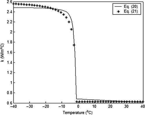
Figure 9 illustrates the behaviour of the thermal conductivity of carrot purée with temperature variation. These curves illustrate an abrupt inclination of the thermal conductivity in a clear-cut interval of temperatures. Thus, when the dependent numerical formularization of the thermal conductivity is used such oscillation cannot be perceived depending on the time step that is used in the simulation. The curve obtained by Equation (21) shown in Figure 3(b) overpredicts the thermal conductivity when compared with the curve shown in Figure 3(a) based on Equation (20).

Figure 9. Thermal conductivity of the carrot purée.

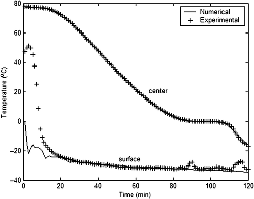
Figure 10 shows the experimental and predicted centre and also the surface temperatures of the carrot purée. These results suggest that the thermal conductivity based on Equations (20) and (21) is a good candidate for simplified predictions of the details of profiles temperatures in the carrot purée. The oscillations verified in the predicted temperature at surface of the carrot purée in freezing initial time suggest that the functions k(T) and H(T) have discontinuities that were not estimated by mathematical model used in the numerical simulations. While the differences between experimental and predicted surface temperatures in freezing final time occur because the experimental ambient temperature is unsteady, however such data was maintained steady during all numerical simulation. It was also observed that the standard error of measurement is higher when lower temperatures are involved.

Figure 10. Profiles of temperature in carrot purée for T_∞ = −38.5°C and h = 400 W m⁻²°C⁻¹.

The optimization algorithms have been analysed by comparing their predicted results with the experimental data and using statistical analysis. Besides the accuracy, the computing cost is another important aspect that relates to the optimization algorithms performance. Table 6 shows the computing time, i.e. the CPU time, for each simulation. All simulations were conducted on a personal computer with Pentium IV, 3.2 GHz processor and 2 GB of Random Access Memory. Generally four factors influence the computing time, the grid resolution, the discretization scheme, the solution for the linear equations system and the configuration of the optimization algorithm. By fixing the first three factors, the difference of computing time is mainly attributed to the optimization algorithm itself. Compared with DE and SOMA, the computing effort of GAF is significantly higher. The DE required the smaller computational time.

Table 6. Computing time (s) required for the optimization algorithms selected in this study.

	Algorithms
Equations	GAF	DE	SOMA
(20)	3091.0	2386.1	2638.7
(21)	3069.7	2305.6	2315.4

5. Conclusion

Three stochastic optimization algorithms of evolutionary computation field, GAF, DE and SOMA, were validated for obtaining the thermal conductivity for carrot purée. These algorithms were selected because of the problem complexity. Numerical results demonstrate that, in general, all three algorithms were suitable for active solution. However, the results described in this article, also show a high degree of reproducibility achieved by SOMA and DE, i.e. smaller variations than GAF.

The SOMA and DE compared with GAF showed better performance and computing effort in this specific application. The results obtained in this work validate the proposed method as a tool to the determination of apparent thermal conductivity in the freezing temperature range. The proposed procedure can be extended to the determination of other thermo-physical properties in different processes like thermal diffusivity and specific heat in drying, wetting, cooling, heating and/or freezing. The determination of thermo-physical properties from an inverse method is an attractive technique both from the experimental and methodological point of view, because of its accuracy and acceptable time for parameters estimation.

Acknowledgements

L. dos Santos Coelho would like to express his thanks to the National Council of Scientific and Technologic Development of Brazil–CNPq–under Grant 309646/2006-5/PQ.

References

- Su, J, and Hewitt, GF, 2004. Inverse heat conduction problem of estimating time-varying heat transfer coefficient, Numer. Heat Transfer Part A 45 (2004), pp. 777–789.
- Loulou, T, and Artioukhine, E, 2003. Optimal choice of descent steps in gradient-type methods when applied to combined parameter and function or multi-function estimation, Inverse Probl. Eng. 11 (2003), pp. 273–288.
- Sawaf, B, Özisik, MN, and Jarny, Y, 1995. An inverse analysis to estimate linearly temperature dependent thermal conductivity components and heat capacity of an orthotropic medium, Int. J. Heat Mass Transfer 38 (1995), pp. 3005–3010.
- Yang, C-Y, 2000. Determination of the temperature dependent thermophysical properties from temperature responses measured at medium's boundaries, Int. J. Heat Mass Transfer 43 (2000), pp. 1261–1270.
- Kim, S, Chung, B-J, Kim, MC, and Kim, KY, 2003. Inverse estimation of temperature-dependent thermal conductivity and heat capacity per unit volume with the direct integration approach, Numer. Heat Transfer Part A 44 (2003), pp. 521–535.
- Znaidia, S, Mzali, F, Sassu, L, Mhimid, A, Jemni, A, Ben Nasrallah, S, and Petit, D, 2005. Inverse problem in a porous medium: Estimation of effective thermal properties, Inverse Probl. Sci. Eng. 13 (2005), pp. 581–593.
- Borukhov, VT, Timoshpol'skii, VI, Zayats, GM, and Tsurko, VA, 2005. Functional identification of the nonlinear thermal-conductivity coefficient by gradient methods. II Numerical modeling, J. Eng. Phys. Thermophys. 78 (2005), pp. 703–709.
- Wood, RL, 1996. Genetic algorithm behaviour in the solution of an inverse thermal field problem, Eng. Comput.: Int. J. Computer-Aided Eng. 13 (1996), pp. 38–56.
- Suram, S, Bryden, KM, and Ashlock, DA, 2005. "An evolutionary algorithm to estimate unknown heat flux in a one-dimensional inverse heat conduction problem". In: Proceedings of the 5th International Conference on Inverse Problems in Engineering: Theory and Practice. Cambridge, UK. 2005.
- Khachf, RA, Bailleut, JL, and Jarny, Y, 2002. "The simultaneous determination of thermal conductivity and heat capacity within an orthotropic medium by using conjugate gradient algorithm". In: IMACS Congress on Scientific Computation, Applied Mathematics, and Simulation. Lausanne, Switzerland. 2002. pp. 1–8.
- Moultanovsky, AV, 2002. Mobile HVAC system evaporator optimization and cooling capacity estimation by means of inverse problem solution, Inverse Probl. Eng. 10 (2002), pp. 1–18.
- Shiguemori, EH, Silva, JDS da, and Velho, HFC, 2002. "Estimation of initial condition in heat conduction by neural network". In: Proceedings of 4th International Conference on Inverse Problems in Engineering. Rio de Janeiro, RJ, Brazil. 2002.
- Silva, CM, and Biscaia, EC, 2004. Multi-objective parameter estimation problems: an improved strategy, Inverse Probl. Sci. Eng. 12 (2004), pp. 297–316.
- Kim, KW, and Baek, SW, 2004. Inverse surface radiation analysis in an axisymmetric cylindrical enclosure using a hybrid genetic algorithm, Numer. Heat Transfer Part A 46 (2004), pp. 367–381.
- Sablani, SS, Kacimov, A, Perret, J, Mujumdar, AS, and Campo, A, 2004. Non-iterative estimation of heat transfer coefficients using artificial neural network models, Int. J. Heat Mass Transfer 48 (2004), pp. 665–679.
- Mendonça, SLR, Celso Filho, RB, and da Silva, ZE, 2005. Transient conduction in spherical fruits: Method to estimate the thermal conductivity and volumetric thermal capacity, J. Food Eng. 67 (2005), pp. 261–266.
- Mariani, VC, de Lima, AGB, and Coelho, LS, 2008. Apparent thermal diffusivity estimation of the banana during drying using inverse method, J. Food Eng. 85 (2008), pp. 569–579.
- Bäck, T, Fogel, DB, and Michalewicz, Z, 1997. Handbook of Evolutionary Computation. Bristol, Philadelphia: Institute of Physics Publishing; 1997, Oxford University Press, NY, Oxford.
- Goldberg, DE, 1989. Genetic Algorithms in Search, Optimization and Machine Learning. New York: Addison-Wesley; 1989.
- Storn, R, and Price, K, 1995. Differential evolution: A simple and efficient adaptive scheme for global optimization over continuous spaces. Technical Report TR-95-012. Berkeley, CA, USA: International Computer Science Institute; 1995.
- Coelho, LS, and Mariani, VC, 2006. Combining of chaotic differential evolution and quadratic programming for economic dispatch optimization with valve-point effect, IEEE Trans. Power Syst. 21 (2006), pp. 989–996.
- Nolle, L, Zelinka, I, Hopgood, AA, and Goodyear, A, 2005. Comparison of an self-organizing migration algorithm with simulated annealing and differential evolution for automated waveform tuning, Adv. Eng. Software 36 (2005), pp. 645–653.
- Michalewicz, Z, Nazhiyath, G, and Michalewicz, M, 1996. "A note on usefulness of geometrical crossover for numerical optimization problems". In: Angeline, PJ, and Bäck, T, eds. Proceedings of the 5th Annual Conference on Evolutionary Programming. San Diego, CA: MIT Press; 1996. pp. 305–312, Cambridge, MA.
- Michalewicz, Z, 1992. Genetic Algorithms + Data Structures = Evolution Programs. New York: AI Series Springer-Verlag; 1992.
- Michalewicz, Z, Logan, TD, and Swaminathan, S, 1994. "Evolutionary operators for continuous convex parameter spaces". In: Proceedings of 3rd Annual Conference on Evolutionary Programming. World Scientific; 1994. pp. 84–97.
- Jong, KADe, 1975. An analysis of the behavior of a class of genetic adaptive systems. Michigan, USA: University of Michigan; 1975, Ph.D Thesis.
- Storn, R, 1997. Differential evolution–a simple and efficient heuristic for global optimization over continuous spaces, J. Global Optim. 11 (1997), pp. 341–359.
- Zelinka, I, and Lampinen, J, 2000. "SOMA–Self-organizing migrating algorithm, Nostradamus". In: Proceedings of 3rd International Conference on Prediction and Nonlinear Dynamic. Zlín, Czech Republic. 2000.
- Vascák, J, 2005. "Evolutionary migration algorithms for scheduling". In: Proceedings of 3rd Slovakian–Hungarian Joint Symposium on Applied Machine Intelligence. Slovakia. 2005. pp. 1–12.
- Oplatková, Z, and Zelinka, I, 2005. "Investigation on Shannon–Kotelnik theorem impact on SOMA algorithm performance". In: Proceedings of 19th European Conference on Modeling and Simulation. Riga, Latvia. 2005. pp. 1–6.
- Incropera, FP, and DeWitt, DP, 1996. Fundamentals of Heat and Mass Transfer. New York: John Wiley & Sons; 1996.
- Fikiin, KA, 1996. Generalized numerical modeling of unsteady heat transfer during cooling and freezing using an improved enthalpy method and quasi-one-dimensional formulation, Int. J. Refrig. 19 (1996), pp. 132–140.
- Mannapperuma, JD, and Singh, RP, 1988. Prediction of freezing and thawing times of foods using a numerical method based on enthalpy formulation, J. Food Sci. 53 (1988), pp. 626–630.
- Scheerlinck, N, Verboven, P, Fikiin, KA, de Baerdemacker, J, and Nicolaï, BM, 2001. Finite element computation of unsteady phase change heat transfer during freezing or thawing of food using a combined enthalpy and Kirchhoff transform method, Trans. ASAE 44 (2001), pp. 429–438.
- Smith, GD, 1985. Numerical Solution of Partial Differential Equations. Oxford, UK: Oxford University Press; 1985.
- Crank, J, 1975. The Mathematics of Diffusion. Oxford: Clarendon Press; 1975.
- Cleland, AC, and Earle, RL, 1984. Assessment of freezing time prediction methods, J. Food Sci. 49 (1984), pp. 1034–1042.