A simple method for tomography reconstruction

Abstract

The problem of reconstructing an image from projections has been extensively studied. Nowadays, the so-called ‘direct methods’ (based on Fourier transform) are the most widely used, mainly because of its low-computational cost. Nevertheless, in some situations old fashion iterative algorithms are more appropriate as is the case of nuclear imaging, where attenuation co-efficents need to be considered in the reconstruction process. In this work, we present an alternative tomography reconstruction method based on the sensitivity of an objective function with respect to small perturbations in the material properties of the problem domain. In particular, we use a simple tomography model to represent the attenuation of 1D projections through 2D slices. Then, we compute the sensitivity associated to the misfit between a boundary measurement and the model solution. Finally, we use this information to devise an iterative algorithm, which allows to reconstruct the attenuation co-efficent defined in the whole domain from exact or noisy synthetic boundary data.

Keywords:

• image projection
• tomography reconstruction
• shape sensitivity

1. Introduction

The inverse problem associated to the reconstruction of the 3D data based on 2D projections has been largely studied. Different alternatives have been proposed over the years 1,2. Early approaches for image reconstruction are based on iterative processes. Although these methods were the most popular in the early days of computed tomography (CT), they present a high-computational cost and its convergence accuracy is compromised by the presence of noise. For these reasons, they became almost completely replaced by direct methods. Nowadays, CT reconstruction is driven by direct methods based on Fourier transform (i.e. filtered back projection–FBP), mainly by the significant computational time reduction.

Nevertheless, there are situations where FBP is not enough and extensions of it or iterative algorithms are more convenient than the basic FBP. For example, in the case of nuclear imaging (single photon emission tomography–SPECT and positron emission tomography–PET), where an internal source is used, direct algorithms do not take into account the absorption of the tissues that surround the illuminating source. This characteristic produces an attenuation on the resulting image that may lead to a misjudgement by the specialist. In the case of PET, different approaches have been used, going from neural networks 3 to random correction 4 with different statistical models, where good results are obtained. For iterative methods, the introduction of attenuation correction may lead to more precise reconstruction results 5. Also, the use of conjugate-gradient preconditioning has brought good results for iterative methods 6,7. Another important feature of iterative methods is the possibility of parallelization 8.

The objective of this work is to present an alternative reconstruction method based on the well-established concept of sensitivity analysis 9. This concept is based on analysing the sensitivity of a specific objective function with respect to small perturbations in the material properties of the problem domain. In particular, we use a simple tomography model to represent the attenuation of 1D projections thought 2D slices. Then, we compute the sensitivity associated to the misfit between a boundary measurement obtained from the real object and the one obtained from the model. Finally, we use this information to devise an iterative algorithm, which allows to reconstruct the attenuation co-efficent defined in the whole domain from boundary data.

This work is organized as follows: first, the simplified tomography model is described and the tomography reconstruction problem is stated. After that, we revisit sensitivity analysis, the addressed objective function and the corresponding sensitivity. Finally, we present the proposed algorithm and some tomography reconstruction results from exact or noisy synthetic boundary measurements.

2. Simple tomography model

When an object (e.g. a body or tissue) is irradiated with an X-ray source, the incident ray is attenuated by two different phenomena: absorption and dispersion. For simplicity, no distinction is made between both effects (considering them together). In order to present the idea, let us consider an object composed by an homogeneous material. If we assume that the object is being illuminated by n rays from the side of the object where the source is located, after an arbitrary period of time during which the object was irradiated, only n + Δn, with Δn < 0, rays were able to pass though the object (where every ray is assumed to have the same energy). In this situation, the following relation is satisfied μ being the rate of photon loss due to both phenomena (which we will call attenuation) and s the variable used to parameterize the path line passed by the ray. Taking Δs → 0, we obtain the following differential equation

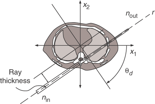
To find the solution of this equation we integrate along the path of the ray through the object using the model presented in Figure 1, considering μ not constant and depending on the spatial variable x (i.e. μ(x), that can be parameterized using s as x(s)). Assuming that the thickness of the ray is small enough, we obtain n_out being the number of photons reaching the sensor for a non-homogeneous object, ds is a differential element along the path line r of the ray. The left-hand side corresponds to a ray integral of a projection. Therefore, measurements like taken from different angles may be used to generate projections of data μ(s). That is,

Figure 1. Ray attenuation path.

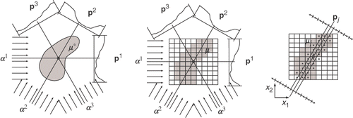
If we consider that the object is being illuminated by m rays in each direction, the expression presented above can be rewritten as α being the intensity of the ray illuminating the object and p the measurement observed at the sensor on the other side of the object. If the object is illuminated in D different directions, d = 1, …, D different projections of μ are obtained, namely (1) In Equation (1), the tomography model is assumed to be continuous. In order to solve this problem computationally, this continuous model needs to be replaced by a discretized one. To do this, the continuous representation of the attenuation co-efficent μ(x) is divided using a regular grid (Figure 2). The values of μ(x) are assumed to be constant on each cell of the grid 10. Then, let μ_i be the constant value of the i-th cell, and N be the total number of cells.

Figure 2. Real obstacle, approximate model and projection example.

In order to obtain the discrete version of the projection data, we cluster the rays j by defining r_j = ∪r_j, where r_j lands on sensor j thus contributing to measure p_j (see Figure 2, projection example), and on each direction m sensors are used. This results in a line running trough the plane spanned by two linearly independent vectors x₁ and x₂ 1. With this in mind, we may express the relationship between μ_i and p_j as following: (2) where M = m * D is the total number of rays in all the projections, and K_ij is a weighting factor that represents the contribution of the i-th cell to the j-th measure (i.e. the intersection between the line and the cell). For simplicity, let us assume the following notation

Therefore, Equation (2) can be rewritten in compact form as following: Note that only a small number of K_ijs are different from zero since only a small number of cells is passed through by any given ray.

3. A tomography reconstruction problem

The tomography reconstruction problem under consideration can be stated as: given the measurement p*, find an approximation μ of the unknown attenuation co-efficent μ* by solving the following equation: (3)

For large values of M and N, different iterative methods exist for solving Equation (3). For example, the so-called ‘method of projections’, first proposed in 11 and reviewed in 12. The computational procedure for finding the solution consists in starting with an initial guess μ⁰ and successively projecting it on the subspaces defined by the rows of K. If a unique solution of the system exists, the iterations will converge to that solution.

Different algorithms based on these ideas have been proposed over the years (ART–algebraic reconstruction technique 13, SART–simultaneous algebraic reconstruction technique 14, etc.).

As mentioned before, in this work we propose an alternative tomography reconstruction method based on sensitivity analysis. For this, a discrete tomography model is used. As will be presented later, in the discrete case, a link between this method and the topological gradient can be established.

In particular, we study the behaviour of a properly defined objective function when the attenuation co-efficents of the object being illuminated is perturbed. With this information, an iterative algorithm is proposed.

4. Sensitivity analysis

Let us consider an objective function Ψ(μ). If we perturb μ (say, μ_T = μ + δμ) we obtain a perturbed objective function Ψ(μ_T), then for small perturbations δμ, the following expansion holds (4) where δμ is such that and the perturbed attenuation co-efficent is that is, the value of μ at cell i was changed from μ_i to μ_T, then meaning that the perturbation is made in one cell. Therefore, gΨ can be recognized as a the sensitivity of the objective function.

In order to minimize the objective function, gΨ · δμ should always be negative. Thus, according to the sign of gΨ, we need to choose the perturbation δμ with the opposite sign. Then, the sensitivity can be used as an indicator providing a descent direction to reduce the value of the objective function. As will be shown in the next sections, this information can be used to develop fast algorithms for tomography reconstruction.

4.1. Objective function definition

Let us now define an appropriate objective function Ψ(μ) for the problem beforehand. As we want to find a μ that produces the best approximation of the observations obtained from the object (p*), we propose Ψ(μ) to be the misfit between p* and the projection data obtained from the model (p). Namely, (5) On the same basis, the perturbed objective function Ψ(μ_T) is defined as (6) From these elements we can calculate an explicit formula for the sensitivity of the objective function.

4.2. Sensitivity calculation

In this fully discrete case, to obtain an expression for the sensitivity we first calculate the total variation of the objective function associated to a perturbation δμ. That is, subtracting Equations (5) and (6), we obtain (7) Then, rearranging this expression and according to Equation (4), the sensitivity is given by (8)

It is easy to notice that gΨ is a vector of N components and that the value g_iΨ indicates the sensitivity of the objective function to a small perturbation in μ_i. It is also important to remark that the sensitivity does not depend on the perturbation, but instead, indicates the direction in which the perturbation should be made for every cell. As observed, in order to reduce the objective function value it is sufficient to take δμ_i with a signal opposite to the one of gΨ at cell i.

As a remark, we may relate the idea discussed in this work with the topological gradient concept. The topological derivative (see 15–19 and references therein), originally conceived for studying topology optimization, has shown promising and interesting results when applied in different image processing problems 20–22. In fact, and as was shown in 23, Equation (8) can be interpreted as the discrete version of the topological gradient associated to the continuous counterpart of the objective function (5) for non-smooth perturbations over the continuous field μ.

5. Numerical results

Using the sensitivity (Equation (8)) as an indicator function, we can devise an iterative algorithm (Algorithm 1) that allows us to find an approximate solution for the above-mentioned problem.

In this case, and for the sake of simplicity in the numerical examples, we assume that a cell might be either intersected or not by a given line. As presented in Figure 1, the sensors have a given thickness. Then, for the computation of the projections, was considered the measure of the intersection of each line with each pixel and multiplied by the attenuation coefficent of that pixel, obtaining the weighting factor K_ij (Equation (2)).

That is, the K_ij coefficent is computed as (Figure 2) where |(·)| is the Lebesgue measure of (·). The measurement vector p* is the input data to the algorithm, obtained from the object being reconstructed. The matrix K is easily computed since the projection directions are known. A short comment should be made on δμ, that does not need to be constant and can be adjusted during algorithm evolution to speed up convergence and provide a more accurate result. At the start of the algorithm, the step size δμ is the same for all the cells and computed as 1/4 of the image average cell absorption (where the value 1/4 was obtained empirically and the average was easily obtained from the projection data). In particular, for the results presented next, δμ was decreased by a factor of 1/2 when, in two consecutive oscillations, g_iΨ changed its sign (interpreted as an oscillation at the i-th cell). Then, the step size is controlled by δμ and only the sign of g_iΨ is used to know the direction in which the perturbation needs to be done.

Table

Algorithm 1: Image reconstruction based on sensitivity analysis
Require: Projection data p*, matrix K, step size δμ and tol.
Ensure: The reconstructed image μ.
set μ^0 = 0, t = 0, Stop = FALSE
while Stop = FALSE do
compute gΨ^t using Eq. (8)
for every cell i do
if giΨ^t < 0 then
else
end if
if sign(giΨ^t)! = sign(giΨ^t−1) then
end if
end for
if |Ψ(μ^t) − Ψ(μ^t+1)| > tol then
t = t + 1
else
Stop = TRUE, μ = μ^t
end if
end while

On the computational cost of the algorithm, each iteration requires two matrix–vector products (N * M) and two vector sums (N) for the sensitivity computation, a run over vector μ^t to find μ^t+1 (M) and the computation of Ψ(μ^t+1) that involves a matrix–vector product (N * M). Then, the computational cost of the algorithm is governed by O(N * M).

5.1. Test 1–Standard reconstruction

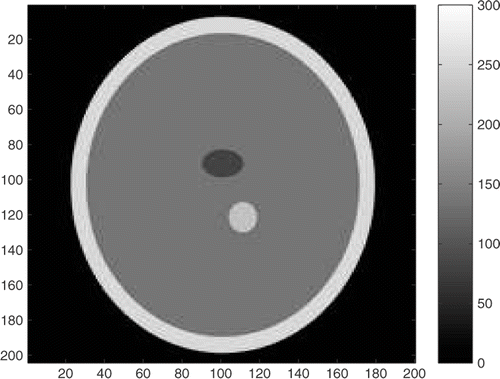
In order to show the performance of the proposed algorithm, some results are shown. The projection data p* was artificially generated from the synthetic data μ*; shown in Figure 3 (256 levels grayscale image of size 200 × 204, with intensities 4, 75, 130, 230 and 250, N = 200 * 204). From this data, different sets of projections were generated for D = 16, 32, 64 and 128. The projection data obtained is also shown in Figure 4.

Figure 3. Original data set used in tests.

Figure 4. Projection data for 16, 32, 64 and 128 directions. The abscissa corresponds to p* for each direction and the ordinate to the d-th direction. The intensity scale is the same for all images.

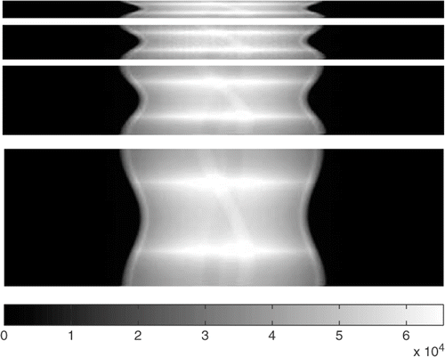
It is important to mention that in this situation a so-called ‘inverse crime’ is being committed, as the same model is being used for the generation of the observations and in the algorithm. For this reason, a second test is driven where the observation data (p*) is perturbed by the addition of different levels of Gaussian noise, a technique widely used in the field for simulating real data.

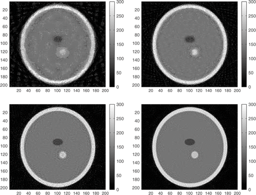
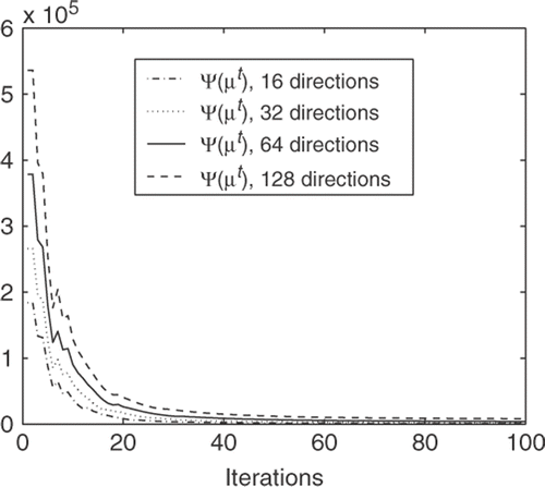
From these projections, an approximation of the original data μ was obtained using the proposed reconstruction method (Algorithm 1). In this case M = (200 + 204) * D was considered, what is enough to fit the projection of the image. As can be seen (Figure 5 for D = 16, 32, 64 and 128 respectively), the reconstructed result presents good quality even for small number of directions.

Figure 5. Results for the gΨ reconstruction method. D = 16, 32, 64 and 128.

In Figure 6, the behaviour of the objective function during the iterative process is presented. As can be seen, the algorithm stabilizes very fast. In approximately 30 iterations the objective function has almost stabilized and very close to zero, meaning that the solution is very close.

Figure 6. Objective function evolution for each case.

5.2. Test 2–Reconstruction with noise

In order to test the robustness of the proposed reconstruction method, in this section some results for different levels of additive noise in the measurement data are presented. The model assumed for the noise polluted measurement pⁿ is (9) where η is a zero mean Gaussian distributed random variable, considered as noise in the signal, and Then, for a signal of strength 100 and p = 5, we consider a 5% noise.

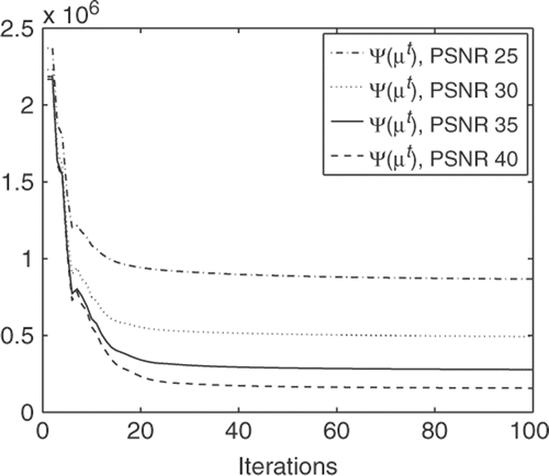
The polluted projection data vector pⁿ was created adding white Gaussian noise to p* with the model described in (9). The noise added was p = 1%, 2%, 3% and 6%. This produces a PSNR (peak signal to noise ratio) of 40 dB, 35 dB, 30 dB and 25 dB respectively. Figure 7 presents the projection data (always with 128 directions) polluted with noise.

Figure 7. Projection data for PSNR 40 dB, 35 dB, 30 dB and 25 dB (128 directions). The abscissa corresponds to p* for each direction and the ordinate to the d-th direction.

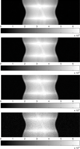
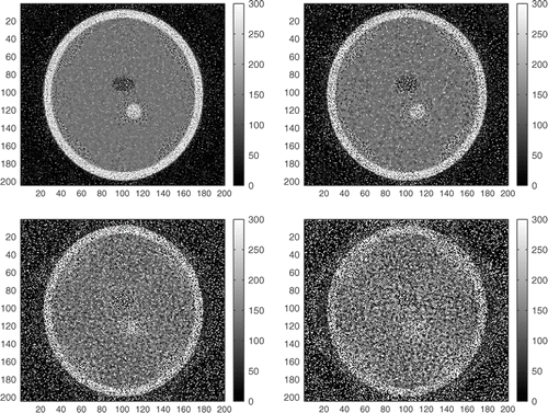
As said before, the polluted data was used to find an approximation of the original data μ with Algorithm 1. As can be seen (in Figure 8 for PSNR 40 dB, 35 dB, 30 dB and 25 dB respectively), the gΨ method obtains good quality results even for intense noise.

Figure 8. Results for the gΨ reconstruction method from noise data with 128 directions for PSNR 40 dB, 35 dB, 30 dB and 25 dB (128 directions).

Figure 9 presents the evolution of the objective function. In this case we see that the objective function does not converge to zero, but still stabilizes in about 30 iterations.

Figure 9. Objective function evolution for reconstruction with noise.

5.3. Test 3–Reconstruction with different discretization

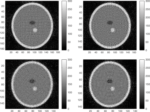
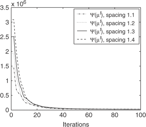
Another way to avoid the inverse crime is to use a different discretization in the reconstructed image than the one coming from the original data. In this third test, the proposed algorithm was used to reconstruct the image with four different discretizations. To do this, the original image is assumed to have cell with constant spacing (i.e. each cell is 1 by 1) and the reconstructed image cells where spaced 1.1 (182 × 185), 1.2 (167 × 170 cells), 1.3 (154 × 157 cells), 1.4 (143 × 146 cells) respectively.

As the projection data is generated according to the size (spacing) of the reconstructed image, different projection data is associated to each configuration (Figure 10) always with 128 directions.

Figure 10. Projection data for different discretizations (1.1, 1.2, 1.3 and 1.4 spacings) and 128 directions. The abscissa corresponds to p* for each direction and the ordinate to the d-th direction.

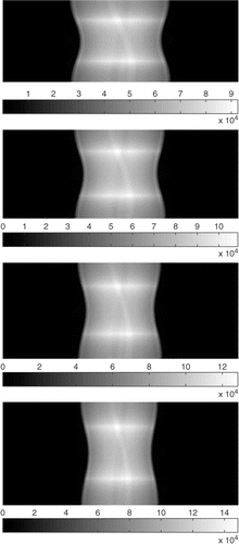
Figure 11 correspond to the reconstructions for spacing 1.1, 1.2, 1.3 and 1.4 respectively. Also in this case, good quality results are obtained. Figure 12 presents the evolution of the objective function for the different spacings. In this case, we may observe that the objective function behaves similar to the first test approximating to zero and stabilizing in few iterations (around 40).

Figure 11. Results for the gΨ reconstruction method for different discretization in the reconstructed image (1.1, 1.2, 1.3 and 1.4 spacings, 128 directions).

Figure 12. Objective function evolution for spacing 1.1, 1.2, 1.3 and 1.4.

6. Conclusions

In this work, the image reconstruction problem was addressed for a simplified tomography model using sensitivity analysis.

To this end, an objective function that takes into account the misfit between the model solution (p) and the exact (p*) or noisy (pⁿ) boundary measurements was used. The model solution is associated to an approximation μ of the attenuation co-efficent of the object μ*. Using the first terms of the asymptotic expansion, it was possible to find an expression for the sensitivity of this objective function to small perturbations in μ. This expression, it was used as an indicator function to find the best places where these perturbations should be introduced, leading to an alternative tomography reconstruction algorithm. Furthermore, the sensitivity of the objective function was used to devise an iterative reconstruction algorithm. The proposed algorithm was used to reconstruct artificial objects considering different number of projections and from exact or noisy synthetic data. In all cases good quality results were obtained, even for considerably large levels of noise and different spacing.

As a final remark, we may state that the presented approach offers an alternative way to treat the tomography reconstruction problem providing easy, fast and robust reconstruction algorithms.

Acknowledgements

This research was partly supported by the Brazilian agencies CNPq/FAPERJ-PRONEX, under Grant E-26/171.199/2003. I. Larrabide was partly supported by the Brazilian agency CNPq (141336/2003-0). The support of these agencies is greatly appreciated.

References

- Kak, AC, and Slaney, M, 2001. "Principles of Computerized Tomographic Imaging". In: Society of Industrial and Applied Mathematics. New York. 2001.
- Natterer, F, 1986. The Mathematics of Computerized Tomography. New York: Wiley-Liss; 1986.
- Bevilacqua, A, et al., 1998. A new approach to positron emission tomography (pet) image reconstruction using artificial neural networks (ann), Int. J. Modern Phys. C 9 (1) (1998), pp. 71–85.
- Yavuz, M, and Fessler, J, 1998. Statistical image reconstruction methods for randoms-precorrected PET scans, Med. Im. Anal. 2 (4) (1998), pp. 369–378.
- Hsiao, IT, and Gindi, G, 2002. Noise propagation from attenuation correction into pet reconstructions, IEEE Trans. Nucl. Sci. 49 (1) (2002), pp. 90–97.
- Fessler, JA, and Ficaro, EP, Fully 3D PET image reconstruction using a Fourier preconditioned conjugate–gradient algorithm, Proc. IEEE Nuc. Sci. Symp. Med. Lm. Cont. 3, pp. 1599–1602.
- Fessler, JA, and Booth, SD, Conjugate–-gradient preconditioning methods for shift variant PETimage reconstruction 8 (5), pp. 688–699.
- Karl, W, et al., 2001. Meeting the computational demands of nuclear medical imaging using commodity clusters, Lecture Notes Comput. Sci. 2074 (2001), pp. 27–37.
- Haug, EJ, Choi, KK, and Komkov, V, 1996. "Design Sensitivity Analysis of Structural Systems". In: Vol. 177 of Mathematics in Science and Engineering Orlando. FL: Academic Press; 1996.
- Rosenfeld, A, and Kak, AC, 1982. Digital Picture Processing. New York: Academic Press; 1982.
- Kaczmarz, S, 1937. Angenaherte auflosung von systemen linearer gleichungeg, Bull. Acad. Pol. Sci. Lett. A 6–8A (1937), pp. 355–357.
- Tanabe, K, 1971. Projection method for solving a singular system, Numer. Math. 17 (1971), pp. 203–214.
- Gordon, R, Bender, R, and Herman, GT, 1970. Algebraic reconstruction techniques (art) for three dimensionla electron microcopy and X-ray photograpy, J. Theor. Biol. 29 (1970), pp. 471–481.
- Andersen, AH, and Kak, AC, 1984. Simultaneous algebraic reconstruction technique (sart): a superior implementation of the art algorithm, Ultrasound Imag. 6 (1984), pp. 81–94.
- Novotny, AA, 2003. "Análise de Sensibilidade Topológica". In: PhD Thesis. Petrópolis, RJ, Brazil: Laboratorio Nacional de Computação Científica; 2003.
- Novotny, AA, et al., 2003. Topological sensitivity analysis, Comput. Methods Appl. Mech. Eng. 192 (2003), pp. 803–829.
- Eschenauer, HA, Kobelev, VV, and Schumacher, A, 1994. Bubble method for topology and shape optimization of structures, Struct. Optim. 8 (1994), pp. 42–51.
- Céa, J, et al., 2000. The shape and topological optimizations connection, Comput. Methods Appl. Mech. Eng. 188 (4) (2000), pp. 713–726.
- Sokolowski, J, and Żochowski, A, 1999. Topological derivatives for elliptic problems, Inverse Probl. 15 (1999), pp. 123–134.
- Auroux, D, Masmoudi, M, and Belaid, L, 2007. "Image restoration and classification by topological asymptotic expansion, in Variational Formulations in Mechanics: Theory and Applications". In: Taroco, E, de Souza Neto, EA, and Novothy, AA, eds. A publication of: International Center for Numerical Methods in Engineering (CIMNE). 2007. pp. 23–42.
- Jaafer Belaid, L, Jaoua, M, Masmoudi, M, and Siala, L, 2008. Application of the topological gradient to image restoration and edge detection, Engineering Analysis with Boundary Elements (2008), doi:10.1016/j.enganabound. 2008.01.004.
- Feijóo, ILarrabideRA, Novotny, AA, and Taroco., EA, Topological derivative: a tool for image processing, Computers & Structures––An International Journal 86 ((13–14)), pp. 1386–1403.
- Larrabide, I, 2007. "Image processing via topological derivative and its applications to Human Cardiovascular System modelling and simulation". In: PhD Thesis. Petrópolis, Brazil: Laboratoório Nacional de Computação Científica–LNCC/MCT; 2007.