Estimating deterministic parameters by Bayesian inference with emphasis on estimating the uncertainty of the parameters

Abstract

Parameter estimation is generally based upon the maximum likelihood procedure which often requires regularization, particularly for non-linear models, and cannot account for nuisance variables or unacceptable regions of parameter values. Bayesian inference can address both difficulties but is computationally expensive and open to questions about the appropriateness of the prior knowledge and when probability densities employed. An approach developed by Banks which is a cross between these methods has been successfully employed with equivalent computational costs. This article compares the three approaches for a simple non-linear test problem.

Keywords:

• parameter estimation
• uncertainty
• confidence intervals
• credible intervals
• Bayesian inference

1. Introduction

The predominant method for estimating parameters is least squares, also known as maximum likelihood, in which a measured response is compared to the predictions of a model whose parameters are sought. This approach not only yields an estimate of the parameters, but also an estimate of the precision of the estimate by way of the classical confidence interval. Most applications of this approach are founded upon the assumption that any noise in the measured response is zero mean and uncorrelated. The method works well when only a few parameters are to be estimated. When several parameters are sought, particularly when the response is a non-linear function of the parameters, it is often found that the approach has difficulties. An alternative is the method of Bayesian inference. This approach is often computationally expensive and requires prior knowledge about the parameters.

A different approach is to employ the least squares approach in such a way that the probability density distributions of the parameters can be determined by an approach suggested by Banks 1. In our use of this approach, we have found that this approach can be used to restrict the parameters to legal values and can handle prior knowledge. When combined with maximum likelihood provides estimates of the parameter uncertainties. In this article, we summarize the basis of the three methods and compare their performance for the estimation of parameters in a lumped mass cooling experiment.

2. The system and its model

Let the measured response of a system be denoted by D (standing for data). The system 𝒮 is modelled by M where t denotes time, and p denotes parameters of the model. This model is presumed to accurately reflect the systems behaviour such that D = M ≡ S(t, P, Θ, 𝒩), where P and Θ represent parameters that are known and to be estimated, respectively, and 𝒩 represents nuisance parameters that affect the model but which we are not interested in estimating. Clearly, the classification of a parameter as belonging to P, Θ or to 𝒩 depends upon the specific situation.

If the measured response is noisy, i.e. σ(D) > 0, then the uncertainty in the parameters, σ(θ), is inversely proportional to the sensitivity ∂M/∂θ. While it is axiomatic that parameters should be estimated only for cases in which the sensitivity is high, there are many cases in which the sensitivities are unavoidably small and the resulting uncertainty in the parameters is large. In these cases, it is important that the uncertainty be accurately assessed.

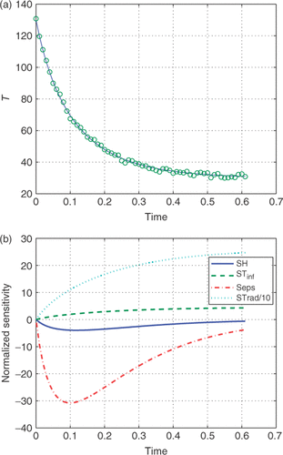
Our test case is the cooling of a lumped mass initially at T_i = 130°C, by convection to the ambient air, T_∞ = 30°C, and by radiation to the surroundings surfaces that are at T_rad = 30°C. The model is: (1) where em is the emissivity, σ is the Stefan-Boltzmann constant, c is the mass capacity, A is the surface area and and . We will look at two cases, em = 0.1 and 0.9 which represent reasonable limits on the radiative transfer. The parameters, H, em and T_rad are to be estimated from T(t) which is contaminated with a uncorrelated noise of zero mean with a SD1 of 1°C. Figure 1 shows the history of the temperature and the normalized sensitivities for em = 0.9. The histories for em = 0.1 are very similar. The sensitivities suggest that T_rad will be best estimated and that em will be estimated with more precision than either H or T_inf.

Figure 1. (a) Temperature histories for emissivity = 0.9. (b) Sensitivity histories for emissivity = 0.9. Available in colour online.

3. Conventional least squares estimation – maximum likelihood

For this model, Equation (1(1) ), a non-linear function of the parameters Θ, let the true value of a parameter be denoted by Θ and the estimated value by . The measurements are presumed to be corrupted by the noise ϵ to give (2) where E[ε] = 0 and cov[ε] = Σ. The estimated values, are those that minimize the functional, L(Θ) (3) where ‖z‖ represents the length of the vector z and (4) Within the linear assumption, provided that the number of readings, N, is sufficiently large it is permissible to evaluate A_j = dM/dΘ at , and the equation is solved iteratively using (5) For d parameters, D and M are [N × 1] vectors, Θ is a [1 × d] row vector and A is a [N × d] matrix. Upon convergence, the estimate satisfies: (6) Using Equation (5a(6) ) it can be shown that: (7) Equations (5b(6) ) and (5c(7) ) represent the generally acceptable desirable state of being an unbiased estimator with minimum variance 2 – i.e. satisfying the Cramer–Rao lower bound 3. In solving Equation (4(5) ) one must know the covariance matrix Σ. Σ can be expressed in terms of the correlation matrix Ω as: (8) where σ_n is the SD of the noise. Ω can usually be obtained by standard statistical analyses 4 taking into account any autocorrelation 5.

At this point, all that one can say about the estimate, , is its value and an approximate value of the SD. Most investigators will then cite the usual equations for confidence limits based on the student t-distribution to give some idea of the range of .

The above development is based upon classical statistics, meaning that is the result of a large number of experiments. Inasmuch as most experiments are performed only a few times at most, Fisher introduced the concept of maximum likelihood which states that the most likely values of parameters are those that maximize the probability of the actual data. Assuming that the errors have a Gaussian distribution, the likelihood is2 (9) found by searching for values of Θ that maximize p(D∣Θ). Since the maximum of p(D∣Θ) occurs when (D − M(Θ))^TΣ⁻¹(D − M(Θ))(≡L) is a minimum, the maximum likelihood method is identical to the weighted least squares method. The maximum likelihood method is probably the single most used method in parameter estimation. In principle, it can be used to estimate both Θ and Σ and any other unknown parameters in the model. If Σ is known, are unbiased. However, estimates of the components of Σ are not unbiased, except in the limit as N → ∞, i.e. asymptotically unbiased 2.

Nuisance variables are parameters that influence the model but which we do not wish to estimate – generally because they often lead to the need for excessive regularization. They may also simply be parameters that we wish to marginalize over (Section 4). Nuisance variables cannot be treated by maximum likelihood. About the best that can be done is to first estimate all parameters, substitute into Equation (7(9) ), and then re-estimate 6.

Applying Equation (4(5) ) to the simulated measurements shown in Figure 1(a) gave the results in Table 1. Note that as the number of parameters to be estimated increases the SD also increases substantially. Most studies report parameters in the form, estimated value ± SD.

Figure 2. (a) Predicted temperature (H + signifies H + σ[H]). (b) Likelihood contours (the squares indicate the estimated values). Available in colour online.

The reader typically interprets the results to mean that the estimates are independent. Using the extreme values, H ± σ[H] and em ± σ[em] to simulate the experimental results, gives the temperatures shown in Figure 2(a). Two choices agree well with the measured temperatures, and two are substantially different. ‘Why’ can be understood by looking at the contours of equal probability shown in Figure 2(b). It is clear that Ĥ and êm are correlated. The reason is easy to understand. The temperature is controlled by the sum of the heat fluxes and an increase in H is compensated for by a decrease in em. Unfortunately, it is rare that authors report in their papers the correlation between the estimated parameters.

Figure 3. Marginal distributions: (a) p(em∣T); (b) p(H∣T). Available in colour online.

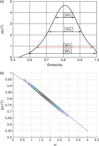
A more disturbing result is that when simultaneously estimating two or three parameters, the SDs are so large that at the 95% confidence level the range of both H and em exceeds the physical limitations, 0 ≤ H, 0 ≤ em ≤ 1 as illustrated in Figure 2(b). Unfortunately the least squares–maximum likelihood method is incapable of incorporating these limits into the estimation process.

Figure 4. Marginal distribution, p(em|T) with 0.75 ≤ emissivity ≤ 1. Available in colour online.

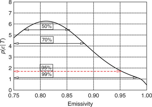
Since the term A^TΣ⁻¹A evaluated at tends to be relatively insensitive to the specific values of θ, the estimated SDs are primarily function of the level of noise and the number of data points regardless of any real limitations.

Table 1. Estimated parameters.

Parameters estimated	E[H]	σ[H]	E[em]	σ[em]	E[Trad]	σ[Trad]
True values	1.0		0.9		303
H	0.9976	0.0050
em			0.8995	0.0061
Trad					302.9	0.201
H, em	1.743	0.6057	0.8087	0.0737
H, Trad	0.930	0.0763			302.6	0.307
em, Trad			0.8916	0.0087	302.7	0.293
H, em, Trad	1.477	0.9256	0.8373	0.1055	302.8	0.460

4. Bayesian inference

The only way to incorporate limits on the parameters is through the use of Bayesian inference which is based on Bayes' equation relating conditional probabilities, illustrated here for two parameters, θ₁ and θ₂ and a response D (10) where (11) π(θ₁) and π(θ₂) are termed the ‘prior’ probabilities and reflect information about θ before the experiment is run. p(θ₁, θ₂∣D) is called the ‘posterior’ probability of θ₁ and θ₂ and reflects how the priors are modified by the experimental data. If the errors are assumed to be normally distributed and a prior which assumes that Θ is normally distributed about a mean of Γ with a variance of V is used, the posterior is: (12) Upon evaluating C, we find that is normally distributed. If the model response is linearized, Equation (3b(3) ), the Bayes' estimator is: (13) with a variance of (14) We see that Bayes' estimators automatically include regularization through the term V⁻¹. For this test case the prior must be such that H and em are restricted to ensure that 0 ≤ H and 0 ≤ em ≤ 1. A variety of different prior probability density forms can be used, e.g. lognormal for H, β for em. Here we present the results only for two very simple and non-informative priors (15) The probability density distribution for em is found by integrating (marginalizing) p(H, em, T_rad∣T) over H and T_rad and is shown in Figure 3 along with the credible intervals. Note that em is appropriately restricted. By plotting the expected value of em given H, i.e. p(em∣H, T) as a function of H, Figure 3(b), we see both the strong correlation and how em is limited to a maximum of 1 as H approaches 0. Table 2 lists the relevant statistics derived from the marginal probability densities. Note that the values of H and em at the point of maximum probability differ from the values in Table 1 because they reflect the integration over the other parameters.

Figure 5. Marginal distribution for em with: (a) 0.75 ≤ em ≤ 1, M=13; (b) 0.75 ≤ em ≤ 1, M=23. Available in colour online.

The distribution shown in Figure 3 was based on a prior that represented no knowledge about em other than 0 ≤ em ≤ 1. The distribution is not unlike the Gaussian distribution that maximum likelihood would produce. Consequently, the statistics given in Table 2 are not significantly different from those given in Table 1. While one may reasonably use non-informative priors about some parameters, it seem that in this test problem it would be easier to place tighter limits. Accordingly, the prior was changed to an non-informative prior over the range 0.75 ≤ em ≤ 1. The resulting distribution is shown in Figure 4 and it differs substantially from that of Figure 3, giving the substantial changes in the statistics shown in the last line of Table 2.

Table 2. Estimated parameters using Bayesian inference at 95% credibility.

Parameters estimated	mode	E[H]	σ[H]	mode	E[em]	σ[em]
True values		1.0			0.9
0 ≤ em ≤ 1	1.727	1.726	0.7572	0.8127	0.8042	0.08718
0.75 ≤ em ≤ 1	1.727	1.438	0.5229	0.8100	0.8438	0.05986

The objections to the use of Bayesian inference are: (1(1) ) that θ are treated as random variables, not unknown constants and (2) the use of unique priors. Bayesians respond to (1) by noting that the probabilities are considered to be subjective, corresponding to our belief about the values of θ and not associated with the frequency of observations. This is consistent with the view of engineers and scientists. Considerable literature is extant on this topic 7. The second objection is a valid criticism of the methodology and any proponent of this approach must be able to show that the prior was a realistic one or that the inference was insensitive to the choice of the prior.

Priors range from the non-informative to the highly specific pdfs. When developing the posterior for the mean of a number of readings, the non-informative priors are: (a) a constant for the mean and (b) 1/σ for the SD. Using these gives the maximum likelihood estimates.

When σ is known, the SD of the mean is , and when the SD is unknown, the estimate of the mean is found to have student-t distribution. This correspondence between Bayesian and classical estimators is not true in general.

While p(Θ∣D) using non-informative priors is a maximum at the maximum likelihood estimates, the marginal distributions of a single parameter, which is found by integration (16) where dΘ_−i signifies that the integration is taken over all parameters except θ_i, will not, in general, have a maximum value at the maximum likelihood estimate.

5. Regularization and non-linearity

Thus far we have concentrated on estimating parameters with confidence limits such that the estimated parameters are in valid ranges. Clearly, this will happen if the SD of the estimates is small.

For Bayesian inference, the validity is enforced through the choice of the priors. A reader who is an unbiased referee may well argue that the prior is not appropriate. One has two options: (a) choose priors that are acceptable to the technical community, (b) demonstrate that the inference is robust, i.e. insensitive to a range of priors. A prior that is uninformative over a realistic range of the parameters, as used in these calculations, is probably acceptable. But one that emphasizes a narrow range of values, e.g. a Gaussian distribution centred about a specific value and with a small SD, is more difficult to support.

The importance of the prior depends upon the accuracy of the experiment. Consider the problem of estimating an average value by making N measurements. If the measurement errors are normally distributed with σ_n and a Gaussian prior with a SD of σ_π is used, the SD of the estimate is given by: (17) As the confidence in the prior increases relative to the experiment, i.e. , either by making the experiment more accurate or by increasing N, and the experiment has contributed little. On the other hand, as , the effect of the prior vanishes.

For maximum likelihood it would appear from Equation (5(6) ), that one simply has to reduce the noise, σ_n, to reduce . Unfortunately the problem is more insidious. A large uncertainty in can occur if the matrix A^TΣ⁻¹A has large elements, i.e. is badly conditioned. In this case, an additional difficulty exists for non-linear problems. From Equation (4(5) ), we see that during the iteration the change, may be so large that the new estimate falls into the illegal area, leading to unacceptable results. Even if one precludes such illegal values, the iteration may stall at the boundaries of the legal values.

Since Bayesian inference does not involve the inversion of A^TΣ⁻¹A, it will be unaffected. The least squares approach relies upon regularization to avoid this problem, but introduces the question of how much and what type of regularization is acceptable 8. Of course the regularization also reduces the accuracy of the estimates.

The sensitivities, Figure 1(b), suggest that T_inf will be most accurately estimated and that there should be no problem estimating H, em, T_rad and T_inf. Yet it turns out that estimating any set of parameters that includes T_rad and T_inf yields a condition number of A^TΣA 10 orders of magnitude greater than any of the other sets. Thus it is not possible to solve Equation (4(5) ) without regularization.

6. Bank's method

In a recent paper, Banks 1 introduced an interesting way to avoid the need to invert A^TΣA yet not relying upon the Bayesian approach with its need to assign priors. Consider defining a sequence of discrete values of a parameter, , often called ‘atoms’ and assigning a probability to each atom. For two such parameters, θ₁ and θ₂ the expected value of the temperature is: (18) where M represents the number of atoms associated with θ and need not be the same for all parameters. Substituting Equation (14(18) ) into the least squares formulation gives: (19) The minimization of L is subject to the constraints (20) (21) applied to each parameter, θ_i. If an atom, say , has the value equal to the estimate derived from the usual least squares approach, with all other values of . If this is not the case, we find that the probabilities at several atoms nearby to the MLE estimate will have non-zero values.

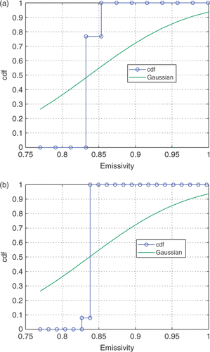
Banks showed that as the spacing between the atoms was decreased, the discrete distribution, i.e. the values of , did not converge to a final static pattern. However, the cumulative discrete distribution did converge. Figure 5 illustrates this procedure for estimating the emissivity.

The uncertainty in the value of is not more than one or two increments in . Once the value of has been determined, then one can evaluate A^TΣ⁻¹A to get the SDs. Since the method does not utilize linearization, it does not require regularization. For one parameter to be estimated, Equation (15(19) ) which is a quadratic and standard constrained quadratic programs can be used. For more than one parameter, it is no longer a quadratic. For two it is a quartic, and the values of must be found using a constrained function minimizer. For this problem with four parameters we used ‘fmincon’ in Matlab.

7. Conclusions

For estimating several parameters of non-linear problem, the least squares approach often requires regularization, leading to questions about the appropriate level and form of the regularizer and introducing uncertainty in the confidence region. In addition, it is not possible to limit the search to acceptable regions or to consider nuisance variables. Bayesian inference can avoid these difficulties, but is computationally expensive and open to questions about the appropriateness of the priors.

Banks' method resolves these problems, but gives no idea about the confidence regions for the estimated parameters. However by combining this algorithm with least squares, one can obtain the confidence regions. As Banks noted, this approach is ‘well posed’, i.e. ‘stable’ in inverse problem terminology. This method can handle nuisance parameters by replacing in Equation (16(20) ) by its integral over any nuisance variable. In addition, it can also restrict parameters by restricting the location of the atoms. However, it cannot handle priors unless more complex constraints are imposed.

Notes

Notes

1. SD denotes standard deviation.

2. p(D∣Θ) denotes the pdf of D given a specified value of Θ.

References

- Banks, HT, 2001. Remarks on uncertainty assessment and management in modeling and computation, Math. Comp. Model. 33 (2001), pp. 39–47.
- Seber, GAF, and Wild, CJ, 1989. Nonlinear Regression. New York: J. Wiley and Sons; 1989.
- Papoulis, A, and Pillai, SU, 2002. Probability, Random Variables, and Stochastic Processes. New York: McGraw-Hill; 2002.
- Shiavi, R, 1999. Introduction to Applied Statistical Signal Analysis. New York: Academic Press; 1999.
- Emery, AF, Blackwell, BF, and Dowding, KJ, 2002. The relationship between information, sampling rates, and parameter estimation models, ASME J. Heat Trans. 124 (6) (2002), pp. 1192–1199.
- Pawatin, Y, 2001. All Likelihood: Statistical Modelling and Inference Using Likelihood. Oxford, UK: Oxford University Press; 2001.
- D'Agostini (Giulio), G, 2003. Bayesian Reasoning in Data Analysis: A Critical Introduction. River Edge, NJ: World Scientific; 2003.
- Engl, HW, 1996. Regularization of Inverse Problems. Boston, MA: Kluwer Academic Publication; 1996.