Application of inverse analysis to illumination design†

^† Preliminary versions of this work were presented in the 10th Brazilian Congress of Thermal Sciences and Engineering (ENCIT 2004) and in the 19th International Congress of Mechanical Engineering (COBEM 2007).

Abstract

This work investigates the application of the inverse analysis to the illumination design of a three-dimensional rectangular enclosure. The illumination design is inherently an inverse problem, in which the design surface is subjected to two conditions–the prescribed luminous flux and null luminous power–while the light sources are left unconstrained. It is considered that all surfaces emit and reflect diffusely, and that the hemispheric spectral emissivities are wavelength independent in the visible region of the spectrum. The illumination design is treated by two different approaches: by an explicit formulation that is regularized by the truncated singular value decomposition due to its ill-conditioned nature; and by an implicit formulation that is treated as an optimization problem using the generalized extremal optimization method, a stochastic algorithm. Both approaches are capable of providing design solutions that satisfy the prescribed luminous flux on the design surface with maximum errors that are less than 3.0%.

^† Preliminary versions of this work were presented in the 10th Brazilian Congress of Thermal Sciences and Engineering (ENCIT 2004) and in the 19th International Congress of Mechanical Engineering (COBEM 2007).

Keywords:

• inverse problem
• illumination design
• radiation exchanges
• regularization
• stochastic optimization

1. Introduction

Illumination plays a fundamental role in several applications, including human activities, manufacturing processes, plants growth and domestic animal reproduction. Various studies have been carried out to provide recommended illumination intensity for many possible applications 1–3. In addition, not only the intensity of light is required, but also its uniformity on the working area. It is the role of the illumination designer to provide a solution for the placement and the power of the lighting devices for adequate illumination of internal spaces where natural light is available or not. Illumination depends on so many parameters that, for a given specification, more than one solution can be proposed. In contrast, it is not uncommon when no satisfactory solution can be found, which may demand modifications in the entire design concept.

Despite being long known that the luminous flux on a given working area not only depends on the power of the light sources, but also on their placements and the effects of the absorbing and reflecting surfaces of the enclosure, the first systematic methods for the analysis and design of artificial lighting were established only in the first half of the twentieth century. Harrison and Anderson 4, 5 proposed an experimental procedure, the now called lumen method, in which the luminous flux on a working plane was determined from a combination of a series of proposed assembling of punctual and continuous light sources. Moon 6 and Moon and Spencer 7, 8 proposed the inter-reflection method for the design of three-dimensional rectangular enclosures having any aspect ratio and being formed by diffuse surfaces. The method presented the advantage of allowing the calculation of the brightness of a surface, accounting for the reflection of light. Due to the complexities of the required calculations, the method requires the use of tables. The lumen method 9 is probably the most widely employed method for the design of illumination, for its algebraic relations provide a rapid, simple procedure to determine the power of the lamps, although the method lacks precision. A more elaborate solution can be achieved by the WinElux code 10, which contains a database of different types of lamps. In spite of their widespread use, both the lumen method and the WinElux code are not, in general, capable of providing solutions that can assure uniformity of luminous flux on the design surface 11.

This work presents the application of the inverse analysis to the illumination design of an enclosure in which a uniform luminous flux, at a specified value, is imposed on a working surface of the enclosure, the design surface. As will be shown, such surfaces are constrained by two boundary conditions: the specified luminous flux and the luminous emissive power, which is zero for surfaces that do not emit light. Two different approaches are proposed. The first one is based on an implicit formulation which relies on the specification of the luminous powers of the light sources, then finding the luminous flux on the design surface. As it would be very difficult to obtain a satisfactory solution with a trial-and-error procedure, searching techniques can be applied to find optimum solutions for the sought parameters. Stochastic-based optimization techniques have proved to be robust for dealing with inverse solutions, for which there is a wealth of methods in the literature. Some recent developments are presented in 12–15. In an alternative approach, the luminous powers required on the light sources are directly found from the two conditions imposed on the design surfaces. This formulation allows some surfaces to be specified on two boundary conditions, while others are left unconstrained. However, for problems that involve radiative exchanges, the problem is described by a Fredholm integral equation of the first kind, known to result in an ill-posed problem, which can be solved only by means of regularization methods 16. Comprehensive reviews of inverse formulation involving radiative exchanges in enclosures are presented in 17–19.

This article combines and generalizes the results of the inverse illumination designs that were previously presented in 20 and 21. The objective is to find the luminous fluxes on the light sources of a three-dimensional rectangular enclosure that satisfy the specified uniform luminous flux on the design surface. All the surfaces that form the enclosure are assumed diffusive and having spectral hemispherical emissivities that are wavelength independent in the visible region of the spectrum (gray surfaces). A zonal-type formulation is applied for the discretization of the radiation exchanges. The two approaches described above are employed. The first one is based on treating the design as an optimization problem, searching for the luminous powers in the light sources that lead to an illumination flux on the design surface that is the closest to the imposed condition. The search relies on the use of the generalized extremal optimization (GEO) algorithm 22. The second approach is based on rearranging the equations to render explicit relations for the luminous power of the light sources. The resulting system of equations is ill-conditioned and is regularized by the truncated singular value decomposition (TSVD) 16, 23. Results are presented to discuss the main characteristics of the two approaches. Although this article considers illumination from incandescent lamps, the methodology can be readily extended to other types of lamps.

2. Physical and mathematical modelling

2.1. Luminous flux and thermal radiation

Incandescent lamps are common sources of light. Their main component is a resistance device that reaches high temperatures (typically around 2900 K) under the passage of electric current. At such temperatures, a considerable amount of thermal radiation is dissipated in the visible region of the wavelength spectrum, 0.4 µm ≤ λ ≤ 0.7 µm. 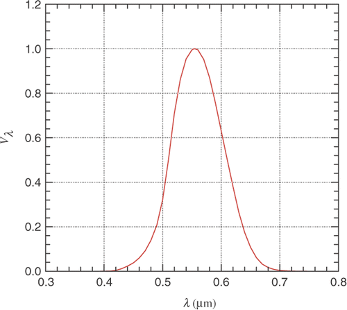The luminous flux, in units of lumens per square metre or lux, can be related to the thermal radiation flux, in units of Watt per square metre, by means of the following relation: (1) where dq^(l) and dq^(w) correspond, respectively, to the luminous flux (lumens per square metre) and to the thermal radiation flux (Watt per square metre) for a specific wavelength λ, within an interval of dλ,C is a conversion factor constant, equal to 683 lm W⁻¹, and V_λ is the so-called photopic spectral luminous efficacy of the human eye, which takes into account the human eye sensitivity to the thermal radiation comprehended in the visible region of the spectrum. As shown in Figure 1, the spectral luminous efficacy peaks with a value of 1.0 for a thermal radiation in the wavelength of 0.555 µm, and then decays monotonically to zero as the lower and upper limits of the visible region, 0.4 and 0.7 µm, are approached. In general, a source of light is composed by radiation covering the entire range of the visible region. In such a case, Equation (1) must be applied to each infinitesimal amount of the spectral energy and then be integrated in the visible spectrum.

Figure 1. Photopic luminous efficacy of the human eye.

2.2. Radiation exchanges in an enclosure

The procedure for the evaluation of radiation heat transfer in enclosures is well established in the literature 24. Light transport can be treated in a very similar way, with the difference that the spectral heat flux must be modified according to Equation (1), and then integrated only in the visible wavelength to lead to the total luminous flux: (2) Applying the energy balance between opaque surfaces of an enclosure leads to the following relations between the luminous fluxes: (3) (4) (5) where is the outgoing luminous flux (radiosity), in lumens per square metre or lux, which takes into account emission and reflection; is the net luminous flux, in lumens per square metre, which accounts for emission minus absorption; is the incident luminous flux, in lumens per square metre; is the blackbody luminous power, in lumens per square metre, which is solely dependent on the temperature; and F_j−k is the view factor between surface elements j and k. To obtain the above relations, it is assumed that all surfaces are gray emitters and absorbers, so that the total hemispherical emissivity and absortivity are equal, that is, . Equations (3–5) apply to enclosures containing non-participating media (such as air), which is representative of the majority of illumination systems. Inverse designs of thermal systems containing participating media have been addressed in 17.

3. Problem definition and formulation

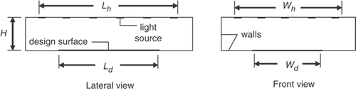
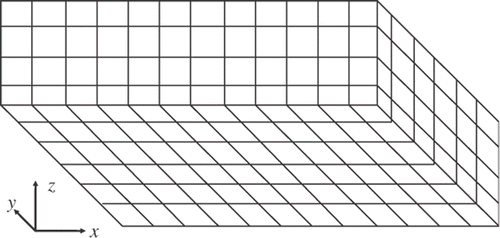
Figure 2 presents a schematic view of a three-dimensional enclosure, formed by surfaces that are diffusive and have spectral hemispherical emissivities that are independent of the wavelength in the visible region of the spectrum. The design surface, where a luminous flux is to be specified, is located at the bottom of the enclosure; the incandescent lamps, the light sources, are located at the top surface. The remaining of the enclosure is formed by walls that do not emit but reflect diffusely the incident light. The length, width and height of the enclosure are designated by L, W and H, respectively. As depicted in Figure 3, the enclosure walls are divided into finite-size square elements, i.e. Δx = Δy = Δz, in which the luminous energy balance will be applied. For designation of elements in the design surface, lamps and wall, indices jd, jl and jw will be used, respectively.

Figure 2. Three-dimensional rectangular enclosure.

In illumination designs, one can impose either the net luminous flux or the incident luminous flux on the design surface, since these quantities are directly related to each other. In this work, it will be imposed a uniform net luminous flux, designated by , but the extension of the methodology to the prescription of the incident luminous flux is immediate. In addition, the temperatures of the elements on the design surface are well below the temperatures for which there is significant amount of thermal radiation in the visible region, so the blackbody luminous power is null, . It follows that two conditions are imposed on the design surface elements: and . For the elements on the wall, one single condition is known, , since they do not emit light. On the other hand, no condition is known for the light source elements. In fact, the conditions on the light sources are to be found from the two specifications on the design surface.

Figure 3. Discretization of the bottom and two side surfaces into finite size elements.

3.1. Implicit formulation

In the implicit formulation, one condition is imposed on each surface element j. For instance, for the design and wall surfaces, the blackbody luminous power, , is set equal to zero; for the light sources, the net luminous flux, , is imposed (alternatively, it could be the blackbody luminous power, ). Then, Equations (3–5) can be arranged to give (6) (7) (8) The last term in Equation (7) arises from the fact that, as depicted in Figure 2, two wall elements jw and jw′ can ‘see’ each other, in which case the view factor between them is not zero. In the above equations, JD, JL and JW correspond to the number of design surface, light source and wall elements, respectively, and the dimensionless luminous fluxes are given by . It follows from this that the dimensionless luminous flux on the design surface becomes Q_r,jd = −1. The negative sign results from the adopted convention that positive heat flux corresponds to energy leaving the system.

Equations (6–8) lead to a system of equations on the unknown outgoing luminous flux Q_o,j of each surface j, with j = jd, jw or jl. This system is in general well-behaved, with the same numbers of unknowns and equations (JD + JL + JW), and can be solved by any standard matrix inversion technique, such as Gaussian elimination, LU factorization, iterative techniques, etc. Once the system is solved for the outgoing luminous fluxes, the unknown condition (the net luminous flux or the blackbody luminous power) can be found for each surface element. For the design surface elements, the net luminous flux can be found by (9) Since the knowledge of one condition is required on each surface element, the implicit formulation can tackle the illumination design by guessing the net luminous flux on each light source, and the solution is run to verify if the imposed net luminous flux on the design surface is attained. Due to the nature of the problem, one should expect to make a large number of guesses to obtain an approximate solution if a trial-and-error approach is employed, unless a searching technique is devised for the selection of the optimum solution. This work considers the latter approach using the GEO algorithm, as described in Section 4.1.

3.2. Explicit formulation

In the explicit formulation, the equations are arranged to render explicit relations for the unknown conditions in the light sources. This advantage comes at the expense of requiring special techniques to solve the resulting system of equations. In this approach, one first needs to combine Equations (3) and (4) for a design surface element jd to relate the outgoing luminous flux, , to the blackbody luminous power and the net luminous flux, and , respectively. Since , the outgoing luminous flux can be found directly from the known net luminous flux, which can be expressed by the following dimensionless relation: (10) Next, Equations (4) and (5), in dimensionless form, and Equation (10) can be applied to each design surface element jd, and then rearranged to provide a system of equations on the dimensionless outgoing luminous flux on the light source elements, : (11) Note that in the above equation, the first term on the right-hand side is known, since it is directly related to the prescribed dimensionless net luminous flux (Q_r,jd = −1). The outgoing luminous flux on the wall elements, Q_o,jw, are unknown, so Equation (7) should be again employed to provide the needed information for the wall elements.

Solving the system of equations formed by Equations (11) and (7) allows the determination of all the unknown outgoing luminous fluxes, so that the net luminous flux on the light source elements can be found from (12) Although this approach provides a direct way to determine the net luminous flux on the light source elements, instead of the searching procedure of the implicit formulation, the system of equations formed by Equations (11) and (7) impose some difficulties. First, the number of equations, JD + JW, is not necessarily equal to the number of unknowns, JL + JW. Second, the system of equations is usually ill-conditioned, and cannot be solved by conventional techniques; in general, it requires regularization. In this article, this will be done with the TSVD, which is described in Section 4.2.

4. Solution of the inverse problem

4.1. Implicit formulation: GEO algorithm

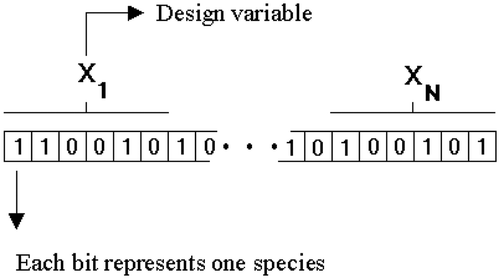
Generalized extremal optimization 22 is an evolutionary algorithm devised to improve the extremal optimization method 25 so that it could be easily applicable to virtually any kind of optimization problem. Both algorithms were inspired by the evolutionary model of Bak and Sneppen 26. In GEO canonical algorithm, the population of species consists of a binary string that encodes the design variables (Figure 4).

Figure 4. Design variables encoded in a binary string.

To each species (bit) is assigned a fitness number that is proportional to the gain (or loss) that the objective function value has in mutating (flipping) the bit. All bits are then ranked from rank 1, for the least adapted bit, to rank N for the best adapted. A bit is then mutated (flipped) according to the probability distribution, defined as P_i(k) = k^−τ, where k is the rank of the bit and τ is the only control parameter. This process is repeated until a given stopping criterion is reached and the best configuration of bits (the one that gives the best value for the objective function) found through the process is returned.

The practical implementation of the canonical GEO algorithm to a function optimization problem is as follows:

1.	Initialize randomly a binary string of length L that encodes N design variables of bit length lj (j = 1, …, N). For the initial configuration C of bits, calculate the objective function value V and set Cbest = C and Vbest = V.
2.	For each bit i of the string, at a given iteration: (a) flip the bit (from 0 to 1 or from 1 to 0) and calculate the objective function value Vi of the string configuration Ci; (b) set the bit fitness as ΔVi = (Vi − Vref). It indicates the relative gain (or loss) that one has in mutating the bit, compared to a reference value. For example, the best objective function value found at the beginning of Step 2; (c) return the bit to its original value.
3.	Rank the bits according to their fitness values, from k = 1 for the least adapted bit to k = L for the best adapted. In a minimization problem, higher values of ΔVi will have higher ranking, and the opposite for maximization problems. If two or more bits have the same fitness, rank them randomly with uniform distribution.
4.	Choose with uniform probability a candidate bit i to mutate (flip from 0 to 1 or from 1 to 0). Generate a random number RAN with uniform distribution in the range [0,1]. If Pi(k) = k−τ ≥ RAN, the bit is confirmed to mutate. Otherwise, choose a new candidate bit and repeat the process until a bit is confirmed to mutate.
5.	Set C = Ci and V = Vi, with i the bit confirmed to mutate in Step 4.
6.	Repeat Steps 2–6 until a given stopping criterion is reached.
7.	Return Cbest and Vbest found during the search.

Note that in Step 4 any bit can be chosen to mutate, but the probability of a given chosen bit be confirmed to mutate is dependent on its rank position. The ones more adapted (with higher rank values) are less prone to have its mutation confirmed and only the least adapted bit (rank = 1) is always confirmed to mutate, if chosen. The probability of mutating the chosen bit is regulated by the adjustable parameter τ. The higher the value of τ, the smaller the chance of a bit (with rank >1) be mutated. The possibility of making moves that do not improve the value of the objective function is what allows the algorithm to escape from local optima.

In a practical application of the GEO algorithm, the first decision to be made is on the definition of the number of bits that will represent each design variable. This can be done by simply setting for each variable the number of bits necessary to assure a given desirable precision for each of them. For continuous variables, the minimum number (m) of bits necessary to achieve a certain precision is given by (13) where and are the lower and upper bounds, respectively, of the variable j (with j = 1, …, N), and d is the desired precision. The physical value of each design variable is obtained through the equation (14) where I_j is the integer number obtained in the transformation of the variable j from its binary form to a decimal representation. Additional information on the method, including how to take into account discrete and integer variables as well as imposing constraints, can be found in 22.

In the illumination design, the problem consists of minimizing the objective function F, which is a measure of the difference between the specified net luminous flux on the design surface, Q_specified = −1.0, and the net luminous fluxes on the design surface that are obtained from a given choice of net luminous flux on the light sources, Q_r,jd, that is, (15) To minimize the above relation, the following procedure is followed:

1.	Define the positions of the light sources;
2.	Define the required precision, d, to determine the minimum number of bits, m, using Equation (13);
3.	Start with a given set of luminous powers for the light sources;
4.	Solve the system of equations described in Section 3.1 to find the net luminous fluxes on the design surface elements, Qr,jd;
5.	Choose a new set of luminous powers on the light sources according to the GEO algorithm;
6.	Repeat from Step 4 until satisfactory solutions for the luminous powers on the light sources are found.

4.2. Explicit formulation: TSVD regularization

Based on the procedure proposed in 17, the following approach is adopted. The outgoing luminous fluxes on the elements located on the walls are initially neglected in Equation (11). Therefore, the unknowns are only the outgoing luminous fluxes on the light source elements, Q_o,jl. Once Equation (11) is written for each of the JD elements that form the design surface, a system with JD equations will be formed. The unknowns are the outgoing luminous fluxes on the JL light source elements. Therefore, the number of equations and the number of unknowns are not necessarily the same, unless JD = JL. In addition, since the problem corresponds to a discrete form of a Fredholm integral equation of the first-kind, one should expect the system of equations to be ill-conditioned. In most cases, such systems should be treated by regularization methods, among them the TSVD is chosen for this solution.

The solution is achieved by means of the following procedure. First, the outgoing luminous flux on each wall element, Q_o,jw, is set equal to zero. Then, the system of equations formed by Equation (11) allows the determination of the outgoing luminous fluxes on the light source elements, Q_o,jl. Next, Equation (7) is applied to each wall element jw to form a system of equations on Q_o,jw. Once the system is solved, the newly computed Q_o,jw are inserted into the system of equations formed by Equation (11), and the procedure is repeated until convergence is achieved. Finally, with the converged values of the outgoing luminous fluxes, Equation (12) is applied to solve for the net luminous flux on each light source element.

The above procedure involves the solution of a system of linear equations on the outgoing luminous fluxes on the light sources, as formed by Equation (11), which can be represented by (16) where matrix A is formed by the view factors between the design surface and the light source elements, F_jd−jl; vector x represents the unknown outgoing luminous fluxes on the light sources, Q_o,jl; and vector b contains the terms on the right-hand side of Equation (11).

For the explicit formulation, the components of the exact solution vector x present steep oscillations between very large positive and negative numbers, and small perturbations cause a much amplified change in the solution. One solving an ill-posed problem should not aim at an exact solution, but rather to impose additional constraints to reduce the size (norm) of x aiming at achieving a smooth solution. Among the regularization procedures, the TSVD is employed here. First, matrix A is decomposed into three matrices: (17) where U and V are orthogonal matrices, and W is a diagonal matrix formed by the singular values w_j. As a consequence, the solution vector x can be computed by (18) As will be illustrated in this problem, the singular values w_j decay continuously to very small values. Since they appear in the denominator of Equation (18), the components of x can present very large absolute numbers. However, the smaller the singular value w_j is, the closer the corresponding vector v_j is to the nullspace of A. In other words, the terms related to the smaller singular values can be eliminated from Equation (18) without introducing a large error into the solution. This is the main idea of the TSVD: only the terms related to the p-th largest singular values are kept in Equation (18), instead of all JL terms. The solution is the vector x with the smallest norm subjected to minimum deviation |A·x − b|. Another feature of the TSVD method is that it can also be applied to the situation where the numbers of unknowns and of equations are not the same, as will be shown in the results section.

Due to the need for regularization of the system of equations, an exact solution is not expected. The following procedure is used for the verification of the solution. Once the net luminous fluxes on the light source elements are obtained, a forward problem is solved where the net luminous fluxes on the light source elements are known, and only the condition is imposed on the design surface (as well as on the walls). The net luminous flux on each element jd of the design surface is then calculated, and compared to the specified heat flux by (19) Once γ_jd is calculated for each element jd in the design surface, the arithmetic average and the maximum errors, γ_avg and , can readily be found.

5. Results and discussion

The case considered in this work consists of a three-dimensional enclosure as shown in the schematic representation in Figure 3. The aspect ratio of the enclosure base is W/L = 0.8; the dimensionless height is H/L = 0.2. The selection of the other dimensions of the enclosure will require a few considerations. First, the design surface ought not to cover the entire extension of the base, since experience has shown that the portions close to the corners would be mainly affected by the reflections from the side walls, not from the luminous radiation from the light source elements on the top surface. Therefore, the design surface dimensions are taken as L_d/L = 0.8 and W_d/L = 0.6. The hemispherical emissivities in the visible light region of the design surface, of the light sources and of the walls are ε_d = 0.9, ε_l = 0.9 and ε_w = 0.5, respectively. The problem is at this point completely defined except for the number and location of the light source elements, which will be considered next.

5.1. Case 1: light sources covering the entire top surface (solution by TSVD only)

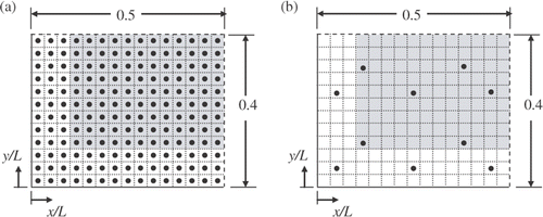
To illustrate the inverse design, it is first considered that the light source elements cover the entire top surface. Figure 5(a) shows the locations of both the light source elements (circular dots) and the design surface elements (shaded area). Due to symmetry, indicated by the dashed lines, only a quarter of the domain needs to be solved: 0 ≤ x/L ≤ 0.5, 0 ≤ y/L ≤ 0.4. One consequence of having the light sources covering the entire top surface is that the numbers of design surface and light source elements (JD and JL, respectively) are not the same. Selecting a grid size of Δx/L = 1/30, which proved to be sufficiently refined to guarantee mesh independence of the results, one finds JD = 108 and JL = 180. Thus, the system of equations formed by Equation (11) will be composed by 108 equations and 180 unknowns.

Figure 5. Locations of the design surface on the bottom (shaded area) and light source elements on the top (circular dots) in one quarter of the bottom and top surfaces for: (a) Case 1; and (b) Case 2. Dashed lines indicate symmetry.

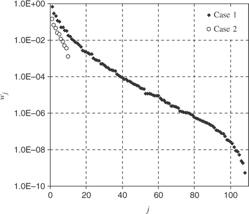
The procedure presented in Section 4.2 is then applied to find the required net luminous flux on the light source elements. Figure 6 shows the singular values of matrix A, under the label Case 1. As typical of inverse design problems, the singular values w_j decay steadily to values that are as small as 10⁻⁹. It should be noted that in the figure only the non-zero singular values are shown; for j > JD = 108, all the singular values are zero. This indicates that this mathematical problem presents infinite exact solutions, in the sense that they satisfy |A·x − b| = 0. To select the exact solution with the smallest norm, one would only need to apply the TSVD method to retain the JD first terms of the series of Equation (18). Taking such a measure, it was observed that the components of vector x had very large absolute values, and alternating positive and negative signals, due to the small singular values that arise in the denominator of the series terms. Since the components of vector x correspond to the outgoing luminous fluxes on the light sources, a positive number, this exact solution has no physical meaning. However, the TSVD can be further explored to keep only the terms of the series corresponding to the p (<JD) largest singular values. In this case, the obtained regularized solution will be no longer exact, but can present a more acceptable behaviour.

Figure 6. Singular values of matrix A: Cases 1 and 2. Index j counts each term of the TSVD decomposition of matrix A in Equation (18).

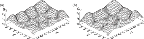
Figure 7 presents examples of regularized solutions for different regularization parameters p = 10 and 8. As seen in the figure, the solutions presented an oscillatory behaviour that are in fact a reminiscent of the steep oscillations of the smallest-norm exact solution (i.e. for p = JD = 108). In general, the smaller the value p is, the smoother the solution will be, although at the expense of presenting a larger error. In fact, for p = 10, γ_avg = 0.6244% and γ_max = 2.7894%; for p = 8, γ_avg = 1.1689% and γ_max = 4.8468%. For p < 8, the solutions presented higher errors, and were considered unsatisfactory. Setting p > 10 led to solutions in which some of the light sources presented luminous powers that were negative. Those solutions are clearly unsatisfactory, and are not presented here. Other regularization techniques, for instance, the modified TSVD (MTSVD) and the Tikhonov methods, can impose side constraints that can assist in avoiding negative solutions. Comparisons between the TSVD and the MTSVD and the Tikhonov methods can be found in 17.

Figure 7. Required net luminous flux distribution on the top surface for different regularization parameters p: (a) p = 10; (b) p = 8. Case 1: light sources covering the entire top surface.

Although this problem could also be tackled with the GEO technique, searching an optimum solution among 180 variables (the net luminous fluxes of the light source elements) would be considerably expensive. However, since the reduction of the light sources is an ever present goal of the illumination design, the GEO technique can naturally be applied to the design concepts that are most interesting. This will be presented in the next section.

5.2. Case 2: reduced number of light sources (solutions by TSVD and GEO)

The solutions obtained and discussed in the previous section illustrate the typical fact that the inverse design technique can lead to a number of approximate solutions, where the final selection can take into account the accuracy and practicality of the solutions. One aspect of the light source configuration of Figure 5(a) is that a very large number of independent light sources would be required (i.e. 4 × 180 = 720 elements for the entire enclosure), which is not practical. The designer will certainly be much more interested on having a smaller amount of light sources. For that matter, the previously selected solution (with p = 10) might provide a hint towards this goal. The fact that only 10 independent terms were enough to provide a solution with acceptable error may be an indication that a solution with only 10 light sources might be enough to satisfy the problem within an acceptable error. Figure 5(b) illustrates a proposed design in which 10 light sources are distributed in one quarter of the top surface. The locations of the light sources roughly coincide with the points of local maximum luminous flux of the solution shown in Figure 7(a).

Since the number of elements on the design remains the same, JD = 108, and the number of light sources is JL = 10, the problem is overspecified; that is, the number of equations is larger than that of unknowns, therefore a problem that can only be solved with some approximation. Figure 6 presents the singular values of matrix A for this case, under the label of Case 2. As seen, the 10 singular values decay to a value in the order of 10⁻³. Keeping all the singular values in the series of Equation (18) provides the smallest norm vector x that satisfies the smallest norm of |A·x − b|. The solution is shown in the last column of Table 1, which indicates the net luminous flux on each element shown in Figure 5(b). In the table, the location of the light sources are indicated by indices i and j to designate the position in the x and y directions, respectively. The resulting luminous flux on the design surface is shown in Figure 8(d).

Figure 8. Dimensionless net luminous flux on the design surface from: (a) GEO¹; (b) GEO²; (c) GEO³; (d) TSVD; Case 2.

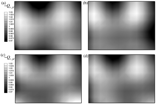
For a reduced amount of light sources, the use of the GEO algorithm becomes more competitive, since the number of variables to be optimized is reduced accordingly. The procedure outlined in Section 4.1 was then applied to find the required net luminous flux on the light source elements. The interval specified in the GEO algorithm was Q_r,jl ∈ [0, 50] for each light source shown in Figure 5(b), with a precision of d = 0.2, so that each variable corresponded to a string composed of m = 8 bits, as given by Equation (13). The parameter τ was varied from 1.25 to 2.25 with a step of 0.25. For each value of τ, 50 different initial configurations C_i were chosen and for each of these configurations, the implicit formulation was run 10,000 times. At the end of the process, 250 different solutions (50 for each different value of τ) were obtained, where the three best results are presented in Table 1: GEO¹–GEO³. Some of the solutions proved considerably different, showing again the typical characteristic of this type of problem, that is, different solutions can satisfy the specified conditions on the design surface. Figure 8(a)–(c) presents the resulting net luminous flux distributions on the design surface for the GEO solutions, which can be compared to the one provided by the TSVD regularization in Figure 8(d). For all solutions, the values of the dimensionless net luminous flux at the design surface are within the interval 0.97 < |Q_r,jd| < 1.03. If a maximum error of 3.0% is considered adequate, all solutions shown in Table 1 and Figure 8 are acceptable.

Table 1. Required dimensionless net luminous flux on the light source elements.

jl	i	j	Qr,jl (GEO^1)	Qr,jl (GEO^2)	Qr,jl (GEO^3)	Qr,jl (TSVD)
1	2	2	0.9804	26.6667	50.0000	17.4009
2	2	8	43.9217	12.5490	10.0000	11.7953
3	4	4	31.5686	25.4902	12.3529	31.1068
4	4	10	24.1176	37.6471	37.4510	36.6861
5	8	2	47.6471	33.3333	31.3725	35.6220
6	8	8	12.1569	19.0196	21.7647	20.8525
7	12	4	4.1176	23.9216	18.8235	15.7124
8	12	10	25.0980	34.5098	31.1765	31.2191
9	14	2	21.3725	18.4314	25.0980	24.5422
10	14	8	25.0980	4.7059	7.4510	9.1672
F, Equation (15)			0.1600	0.1553	0.1408	0.1325

Table 1 also presents the value of the objective function F, defined by Equation (15), for each solution. Note that the result obtained with the TSVD regularization method was the one with the smallest error. For a given level of regularization of the system of equations, or alternatively for a given level of perturbation of the original problem, the TSVD method selects the smallest norm solution that leads to the smallest value for the error function. However, depending on the level of regularization, the solution via the optimization method may present smaller errors.

Comparing their computational efforts for the same computer machine, while the TSVD regularization of the inverted system of equations required only a few minutes, the use of GEO algorithm required a few days, since the implicit system of equations had to be solved multiple times. However, this computation time can be greatly reduced with an increased experience in the selection of the optimum parameters in the GEO algorithm, and with the use of parallelization. Another attractive aspect of an optimization technique such as the GEO algorithm is that it allows the choice of a variety of solutions (as shown in Table 1), and can be extended to find the optimum position of the light sources, contrarily to the regularization techniques, for which it would be very difficult to treat the geometry parameters as unknowns of the problem. Also, in the case of the solutions via the regularization of the matrices that describe the inverse relations, it is often found negative values for the luminous power of the light sources, which is not physically acceptable. On the other hand, when treating the inverse design as an optimization problem, since the interval for the values of each luminous power of the light sources are defined by the designer, reaching non-physical results is avoided.

6. Conclusions

This work considered an inverse analysis in which the net luminous fluxes on the light source elements were determined to satisfy a specified uniform luminous flux on the design surface. The problem was treated by both the implicit and explicit formulations. In the first approach, the solutions were sought by a recently developed optimization algorithm named GEO, in which a number of propositions for the net luminous fluxes on the light sources were selected, tested and compared to find the best answers. On the other hand, the explicit formulation attempted to find the solution in a single step, but led to an ill-conditioned system of equations, which was regularized by the TSVD.

Two design cases were studied. In the first case, it was considered that the light source elements covered the entire top surface. Since the large number of unknown parameters would demand a very large computational time for a stochastic method such as the GEO technique, only the TSVD regularization of the explicit formulation was applied. The selected solution was obtained when keeping only the first 10 terms of the series that forms the solution vector. In the second case, it was proposed an inverse design in which only 10 light source elements were set at the top surface. This design problem is closer to practical applications, since it requires a reasonable number of light sources, and was solved by both the TSVD regularization and the GEO algorithm. The obtained solutions presented errors that were <3.0%, a precision that can hardly be attained with the usual techniques of illumination design.

Although the GEO algorithm requires considerably more computational effort than the TSVD regularization of the explicit formulation, it presents some important features for the inverse design. First, the method avoids the non-physical solutions that can arise from explicit formulation, even after the regularization. Second, the GEO algorithm presents a great deal of flexibility, and can deal with the problem of finding the optimum position of the light sources, which would be very difficult with an explicit formulation by setting the positions as unknowns. Other important implementations towards an even more accurate representation of actual illumination systems are the consideration of non-gray surfaces and non-diffuse lamps.

Acknowledgements

F.H.R. França thanks CAPES for the support under the program CAPES/UT-AUSTIN, No. 06/02, and CNPq through research grant 304535/2007-9. A.J. Silva Neto acknowledges the support provided by CNPq, through research grant 300171/97-8, FAPERJ and CAPES.

Notes

^† Preliminary versions of this work were presented in the 10th Brazilian Congress of Thermal Sciences and Engineering (ENCIT 2004) and in the 19th International Congress of Mechanical Engineering (COBEM 2007).

References

- Boast, WB, 1953. Illumination Engineering. New York: McGraw-Hill; 1953.
- Lewis, PD, and Morris, TR, 1998. Responses to domestic poultry to various light sources, World Poultry Sci. J. 54 (1998), pp. 7–25.
- Mark, S, 2000. The IESNA Lighting Handbook. New York: Illuminating Engineering Society of North America; 2000.
- Harrison, W, and Anderson, EA, 1916. Illumination efficiencies as determinated in an experimental room, Trans. Illum. Eng. Soc. 11 (1916), pp. 67–91.
- Harrison, W, and Anderson, EA, 1920. Coefficients of utilization, Trans. Illum. Eng. Soc. 15 (1920), pp. 97–123.
- Moon, P, 1941. Interreflections in rooms, J. Opt. Soc. Am. 31 (1941), pp. 374–382.
- Moon, P, and Spencer, DE, 1946a. Light distribution in rooms, J. Franklin Inst. 242 (1946a), pp. 111–141.
- Moon, P, and Spencer, DE, 1946b. Light design by the interreflection method, J. Franklin Inst. 242 (1946b), pp. 465–501.
- IESNA–Illuminating engineering society of North America, 2000. Rea, Mark Stanley, ed. The IESNA Lighting Handbook: Reference & Application. New York: IESNA; 2000. pp. 9.28–9.51.
- EEE – Empresa de Equipamento Elétrico SA, 2002. Portugal: Águeda; 2002, Available at www.eee.pt.
- Seewald, A, 2006. "Inverse design analysis with non-gray surfaces: An approach for illumination design". In: Masters Degree Thesis. Graduate of Mechanical Engineering, Federal University of Rio Grande do Sul; 2006.
- De Sousa, FL, Soeiro, FJCP, Silva Neto, AJ, and Ramos, FM, 2007. Application of the generalized extremal optimization algorithm to an inverse radiative transfer problem, Inverse Probl. Sci. Eng. 15 (2007), pp. 699–714.
- Cuco, APC, Neto, AJSilva, Velho, HFCampos, and Sousa, FLDe, 2008. Solution of an adsorption problem with an epidemic genetic algorithm and the generalized extremal optimization algorithm, Inverse Probl. Sci. Eng. ifirst (2008), DOI: 10.1080/17415970802083201.
- Galski, RL, Sousa, FLDe, Ramos, FM, and Neto, AJSilva, Application of a GEO + SA hybrid optimization algorithm to the solution of an inverse radiative transfer problem, Inverse Probl. Sci. Eng., Accepted for publication.
- Jr, JLugon, Neto, AJSilva, and Santana, CC, A hybrid approach with artificial neural networks, Levenberg–Marquardt and simulated annealing methods for the solution of gas-liquid adsorption inverse problems, Inverse Probl. Sci. Eng., Accepted for publication.
- Hansen, PC, 1998. Rank-Deficient and Discrete Ill-Posed Problems: Numerical Aspects of Linear Inversion. Philadelphia: SIAM; 1998.
- França, F, Howell, J, Ezekoye, O, and Morales, JC, 2002. "Inverse design of thermal systems". In: Hartnett, JP, and Irvine, JP, eds. Advances in Heat Transfer. Vol. 36. San Diego: Academic Press; 2002. pp. 1–110.
- França, FHR, and Howell, JR, 2006. Transient inverse design of radiative enclosures for thermal processing of materials, Inverse Probl. Sci. Eng. 14 (2006), pp. 423–436.
- Daun, K, França, FHR, Larsen, M, Leduc, G, and Howell, JR, 2006. Comparison of methods for inverse design of radiant enclosures, ASME J. Heat Transfer 128 (2006), pp. 269–282.
- Schneider, PS, and França, FHR, Inverse analysis applied to an illumination design. Presented at Proceedings of the 10th Brazilian Congress of Thermal Sciences and Engineering. ENCIT, Rio de Janeiro, 2004, Brazil.
- Mossi, AC, Schneider, PS, França, FHR, Sousa, FLDe, and Neto, AJSilva, Application of the generalized extremal optimization (GEO) algorithm in an illumination inverse design. Presented at Proceedings of the 19th International Congress of Mechanical Engineering. COBEM, Brasília, 2007, Brazil.
- De Sousa, FL, Ramos, FM, Paglione, P, and Girardi, RM, 2003. New stochastic algorithm for design optimization, AAIA J. 41 (2003), pp. 1808–1818.
- Hansen, PC, 1990. Truncated SVD solutions to discrete ill-posed problems with ill-determined numerical rank, SIAM J. Sci. Stat. Comp. 11 (1990), pp. 503–518.
- Siegel, R, and Howell, JR, 2002. Thermal Radiation Heat Transfer. Washington: Hemisphere Publishing Corporation; 2002.
- Boettcher, S, and Percus, AG, 2001. Optimization with extremal dynamics, Phys. Rev. Lett. 86 (2001), pp. 5211–5214.
- Bak, P, and Sneppen, K, 1993. Punctuated equilibrium and criticality in a simple model of evolution, Phys. Rev. Lett. 71 (1993), pp. 4083–4086.