Abstract
The technique of solving linear steady-state and transient inverse problems aimed at retrieving an unknown heat transfer coefficient (HTC) is proposed. The idea is to approximate the temperature field by a linear combination of known auxiliary temperature fields. Each of these fields is evaluated by assuming that the unknown boundary temperature (heat flux) is described by a compact support, low-order trial function. The unknown coefficients of this linear combination are determined from the least square fit to the measured temperatures employing the modified Levenberg–Marquardt (LM) method. Once the boundary temperature and heat flux are retrieved, the HTC is determined from its definition. The auxiliary fields are evaluated using an arbitrary numerical or analytical technique. The sensitivity coefficients of the problem can readily be obtained by sampling the auxiliary fields at sensor locations. The values of the sensitivity coefficients used in the LM procedure need to be determined only once, before entering the iterative least squares procedure. Piecewise linear or stepwise functions were used to approximate the spatial and temporal variation of the retrieved heat flux and temperatures. The technique has been applied to reconstruct HTC for so-called time-to-arrival measurements technique with narrow band thermochromic liquid crystal used as temperature sensors. The idea behind this approach is to monitor the time at which a measuring point reaches a characteristic temperature. The developed technique has been used to retrieve the HTC for impingement cooling of the simplified piston of a car engine.
Nomenclature
| Latin: | = | |
| A | = | –error amplitude, s |
| d, D | = | –diameter, m |
| h | = | –heat transfer coefficient, W/m2K |
| I | = | –number of sampling points (sensor locations) |
| j | = | –sensitivity coefficient |
| J | = | –sensitivity matrix |
| K | = | –number of spatial trial functions |
| N | = | –spatial trial function |
| M | = | –temporal trial function |
| q | = | –heat flux, W/m2 |
| r | = | –vector coordinate, m |
| R | = | –residual |
| t | = | –time, s |
| T | = | –temperature, K |
| U | = | –number of temporal trial functions |
| Greek: | = | |
| Γ | = | –boundary |
| Φ | = | –minimized objective function, K2 |
| Θ | = | –auxiliary temperature field, K |
| Ω | = | –domain |
| Subscripts: | = | |
| 0 | = | –initial |
| a | = | –activation |
| E | = | –boundary where the boundary conditions are known |
| m | = | –mean |
| mod | = | –from model |
| f | = | –free stream |
| R | = | –boundary where heat transfer coefficient is to be retrieved |
| z | = | –number of a spatial zone |
| Superscripts: | = | |
| = | –retrieved | |
| = | –measured | |
| = | Variables set in boldface are vectors or matrices |
1. Introduction
The jet impingement technique consists in directing a jet flow from a nozzle to a target, typically a solid surface. Many types of nozzle and target surface geometries are encountered in practice. The momentum of the jet destroys the boundary layer at the surface, leading to intensive heat exchange. The efficiency of this heat transfer arrangement makes jet impingement a popular method of intensive cooling and heating. Drying of textiles, cooling of electronic packages, cooling of slabs in steel industry, car or aircraft engine cooling Citation1 are just few examples of applications of the jet impingement technique encountered in the industry.
Proper determination of the HTC for that kind of cooling is difficult. Some theoretical methods of evaluating the HTC for jet impingement are available Citation2–5. The underlying analysis bases on boundary layer formulation and the applicability of the results is fairly limited. A more universal, yet significantly more time consuming, approach is to solve the set of conservation equations encompassing mass, momentum and energy transfer in the jet, the surrounding fluid and the target surface. Computational fluid dynamics (CFD) solutions of such problems are reported in the literature Citation6–8. To handle turbulent flows, constituting a vast majority of impingement flows encountered in practice, additional empirical closure equations need to be included in the model. Both Reynolds averaged Navier Stokes and large eddy simulation methods are used Citation9,Citation10. The results strongly depend on the applied closure equations. A high temperature and velocity gradient of the shearing flow not only requires very dense numerical meshes but also deteriorates the convergence rate. As a result, the execution time of the CFD simulations is, even in the case of one phase systems, prohibitively long. Simulation of liquid jets in a gaseous atmosphere is much more complex, due to multiphase flow, presence of free surface and breakup mechanism.
The alternative method of retrieving the HTC is the application of the inverse analysis. The computational load of this technique is typically low, but expensive and time-consuming experiments are necessary. The advantage of this approach is its accuracy, which may be significantly higher than that of CFD simulations. Inverse technique has been used to reconstruct heat flux at stagnation point, e.g. Citation11.
The idea behind the inverse analysis is to find the best fit between the model and the experiments. The model equations are obtained by solving appropriate boundary value problems with assumed values of the unknown parameters. Minimization of the discrepancy between the measurements and the model leads then to an iterative optimization (least squares) problem. When realistic geometry is involved, the model equations are solved using a numerical solver and the execution time may be long. It is customary to solve the best-fit problem using gradient optimization methods. In this case, the evaluation of the sensitivity (Jacobian) matrix is far more expensive than the solution of the model equations. Inverse analysis leads thus often to intensive numerical calculations. Acceleration of the procedure can be achieved by simplifying, at the expense of the accuracy, the geometry and/or boundary conditions (BC) of the original boundary value problem. The aim of this article is to speed up the inverse analysis without affecting the accuracy. The developed technique is used to solve a practical problem of determining the HTC of an oil jet cooled car engine piston.
The optimization solver employed in this article is the modified Levenberg–Marquardt (LM) Citation12 algorithm. The technique is known for its regularization properties mitigating the ill-posedness of the inverse problem Citation13. The solution of the model equation and the evaluation of the sensitivity coefficients were accomplished using MSC.Marc, a commercial finite element method (FEM) code. The calculation of one column of the sensitivity matrix requires a solution of one properly defined boundary value problem. When multiply load option of the FEM code is invoked, the execution time can be significantly reduced. It is important to mention that the entire sensitivity matrix is evaluated only once, before entering the iterative loop. This feature drastically reduces the execution time of the proposed technique.
The article concerns the reconstruction of the heat transfer coefficient (HTC). Its distribution is found indirectly by retrieving the boundary temperature and heat flux. The HTC is then calculated from the definition of the Robin BC.
The developed method has been validated using pseudo measurements obtained by a solution of known direct problems. To simulate the measurement error the results of the pseudo measurements have been laden by stochastic error of pre-defined amplitude.
2. Experiment
Standard temperature sensors measure the temporal variation of the temperature. Sometimes, however, it is easier and more accurate to measure the time a given point needs to reach a pre-defined temperature Ta, known as the activation temperature. The time instant ta at which this happens is referred to as the activation time (). This type of measurements is called time-to-arrival and is typical for narrow band thermochromic liquid crystals (TLC) and phase change material (PCM).
Figure 1. Temperature history of a selected point. Definition of the activation time and temperature.
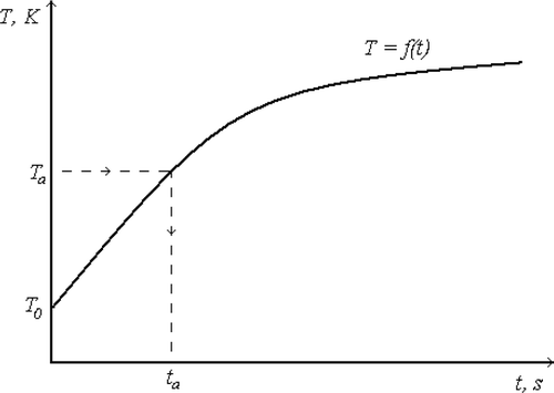
The HTC estimation technique proposed in this article uses this kind of measurement. There are two disadvantages to this method. The full information about the temporal changes of the temperature is sampled at one instant. Moreover, the knowledge of the spatial distribution of the temperature at a given time instant is incomplete. The information is limited to points that have actually reached the activation temperature. This means that for some time instances no information about the temperature field might be available. These disadvantages strongly limit the number of possible applications for that kind of measurement. The advantage of it is that only a small amount of information is acquired and needs to be stored during the process, making the practical implementation of this procedure much easier. Moreover, when compared with standard TLC thermography, the temperature values are measured more precisely.
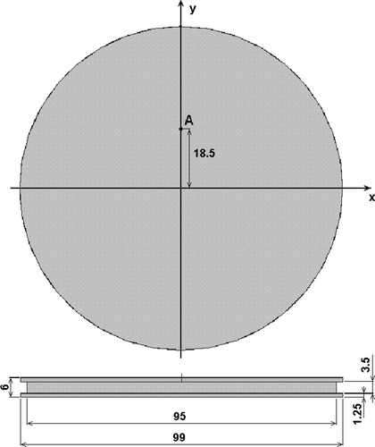
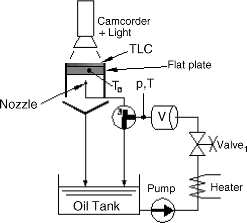
The aim of the research was to determine the variation of HTC on the surface of a car engine piston cooled by an oil jet. A simplified model of the piston was a circular aluminum flat plate with a side neck (). The material properties of the plate were provided by the manufacturer. The oil impinges bottom surface of this plate at point A. The test rig used in the project is shown in .
In the oil tank 20 litres of synthetic engine oil was stored. At the beginning of the experiment the oil was pumped with a maximum pressure of 3MPa back to the tank flowing through a 1.5 kW electric heater and three valves: valve1 controlling the flow rate, a three-way valve 3w used to redirect the flow. Once the temperature of the oil reached 100°C, the three-way valve was turned to redirect the oil flow to the nozzle. The hot oil jet leaving the nozzle impinged the plate, initially at room temperature. As a result, the plate was gradually heated up. The oil was then gravitationally discharged back to the oil tank. The role of valve1 was to control the flow rate. The measuring devices applied in rig were the following:
| • | oil pressure p–Keller relative probe, | ||||
| • | oil temperature T–resistance temperature detection sensor, | ||||
| • | volumetric flow rate V–a gear type device. | ||||
The camcorder started to record the pictures of the test surface at the very moment when the three-way valve redirected the flow of oil to the nozzle. In the course of the test, the pressure of the oil, its temperature and flow rate, are acquired and stored along with a sequence of bitmaps of the TLC. The test terminated when the temperature exceeded the TLC activation temperature over the entire test surface.
The data processing started with postprocessing of the bitmaps. The aim was to evaluate the time-to-arrival matrix, i.e. for each pixel of the bitmaps the time necessary to reach the red peak intensity temperature (40.9°C) was determined. shows the sample bitmaps after 8.4 s from the start of the test and the relative map of the time to arrival. The images show, as expected, that the peak value of the heat flux is at the impingement region where the surface temperature grows quickly.
Figure 4. Acquired picture of the TLC after 8.4s (left) and the distribution of the time to arrival during the entire experiment.
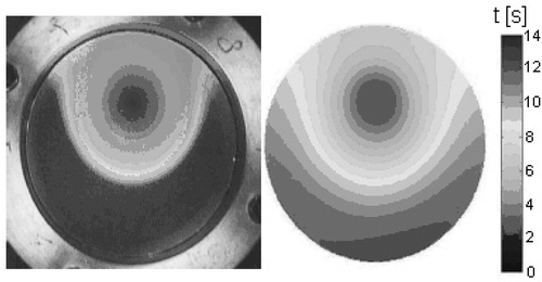
The measurement error results from the uncertainty of the time measurements, localization of the red peak intensity in time and pixel location. The uncertainty of 0.04 s, which corresponds to one frame of recorded movie, is assumed to be the error of time measurements and red peak intensity localization. The spatial resolution of the picture is high, and thus the positioning error caused by location uncertainty is assumed be of the order the sampling time. That gives a coarse assessment of the total time measurement in the order of 0.12 s.
3. Temperature field as a function of the unknown boundary heat flux
As already mentioned, in order to reconstruct the HTC both temperature and heat flux distributions on the boundary are retrieved. The derivation of the technique of retrieving boundary flux is presented first. A more detailed description of the technique with the theoretical background based on Green's function can be found in Citation15. For the sake of simplicity, steady state temperature field is considered first.
The computational domain Ω is bounded by a surface Γ divided into two parts. On the first part ΓR the heat flux qR is unknown. On the remaining portion of the boundary denoted by ΓE, the BCs are known. The problem is linear, internal heat generation can be accounted for. Resorting to the linearity of the problem, the temperature at arbitrary point r can be expressed as a sum of two temperature fields:
(1)
where the TE is the temperature field corresponding to the zero flux prescribed on ΓR and the BC on ΓE and the internal heat generation as in the original problem. As all data needed to evaluate this temperature field are known, TE can be determined solving a direct problem using any suitable method.
The second temperature field TR corresponds to homogeneous BCs on ΓE, zero internal heat generation and actual heat flux on boundary ΓR. Homogeneous BCs on ΓE are generated from the original ones just by dropping the known right-hand side. It means that zero temperature is assumed for Dirichlet BCs and insulation for Neumann BCs. For the convective (Robin) BC, heat exchange with a fluid of zero temperature is considered, with the HTC remaining intact. Temperature field TR is unknown as it depends on the distribution of the heat flux on ΓR. To evaluate this field the searched for heat flux is expressed as a linear combination of known trial functions Nk
(2)
where Nk are known approximation (trial) functions and qk stand for unknown scalars. Coefficients qk may not have any physical meaning, but it is advantageous to interpret them as values of heat flux at certain points. The trial functions can then be seen as functions of local support analog to shape functions arising in FEM and BEM techniques Citation1.
Approximation (2) and the linearity of the problem lead to a simple formula linking TR with the unknown coefficients qk
(3)
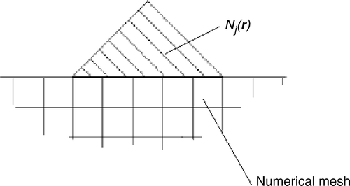
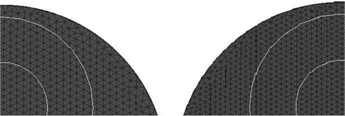
where Θk is a temperature field obtained taking the heat flux on ΓR as equal to Nk, keeping the BCs on ΓE homogeneous and neglecting the internal heat generation. As all data necessary to evaluate Θk are known, these temperature fields can be determined uniquely by solving a direct problem using suitable solution technique. In the case the direct (forward) problems are solved using numerical methods, to maintain appropriate accuracy fine meshing of the entire domain, including boundary ΓR is required. In such cases, the intervals used in the definition of the trial functions Nk should be much coarser than the grid applied in the forward problem ().
Substituting Equation (3) into Equation (1) produces
(4)
Sampling Equation (4) at a sequence of points ri, i=1, 2, …, I produces a matrix equation
(5)
where the entries of the matrices and vectors are defined as
(6)
(7)
(8)
(9)
Defining the sensitivity coefficient jki as the derivative of the temperature at a given point ri, with respect to the unknown parameter qk it can be readily seen that this quantity is just the entry of the J matrix and, at the same time, the sampled auxiliary temperatures Θk(ri) entering Equations (3) and (4).
(10)
For transient fields the temporal variation of the temperature needs to be accounted for. The approximate variation of the unknown heat flux on boundary ΓR is then written in the form
(11)
where M is a known trial function depending solely on time and
is unknown parameter describing the temporal and spatial distribution of the heat flux on ΓR. The temporal trial functions are completely analogous to their spatial counterparts, i.e. they vanish for times outside a user defined interval.
Introducing a function Qp(r, t) = Nk(r)Mu(t) with the index p defined as p = K(u − 1) + k brings Equation (11) to a more compact form
(12)
The linearity of the problem yields a relationship analogue to Equation (4),
(13)
where TE is the temperature field corresponding to the original: initial condition, intact BCs on ΓE and original distribution of internal heat sources. The heat flux on ΓR is zero. Temperature field Θp corresponds to homogeneous initial conditions, homogeneous BCs on ΓE and heat flux on ΓR equal to Qp.
Evaluation of TE and Θp is accomplished by solving a well-defined forward problem with all data known. These forward problems are most often solved using numerical time stepping procedures. To maintain accuracy, the time increment employed in the forward problems should be small. On the other hand, in order to mitigate the ill-posedness of the inverse analysis, the temporal intervals used to define M, should be in such cases much larger.
In the problem at hand, only one time-dependent function has been used (U=1). The multi-step procedure is discussed in Citation15. Sampling Equation (13) at a set of points and time instants produces a linear dependence between the temperatures and the unknown parameters. The shape of the matrix equation is identical to Equation (5), but the entries are now defined as
(14)
(15)
(16)
(17)
where s = I(w − 1) + i and w stands for subsequent time interval at which the temperature field is sampled.
The unknown parameters stored in vector q can be obtained from the least square fit of model Equation (5) and a set of temperatures measured at sampling points and times. With standing for a vector of measured temperatures, the least squares problem is defined as
(18)
Once the problem is solved, the distribution of the heat flux on ΓR can be found from Equation (12). Resorting the necessary conditions for minimum, the problem can be recast into a solution of a over determined set of linear algebraic equations. Ill-posedness of the set requires special techniques of solving both the original least squares problem and the resulting over determined set of equations.
4. Temperature field as a function of the unknown boundary temperature
To retrieve the temperature on boundary ΓR, the temperature in the domain should be expressed as a function of the unknown temperature distribution. The technique of deriving this relationship is completely analogous to that used in the previous section. The starting point is the approximation of unknown temperature TR using a formula.
(19)
where the unknown parameters Tp are analogue of qp arising in Equation (12). The trial functions Nk(r) and Mu(t) entering the definition of Qp may be distinct from those used when approximating the unknown heat flux on ΓR.
From the linearity of the problem, the temperature field can be expressed as
(20)
where TE is the temperature field corresponding to the original: initial condition, intact BCs on ΓE and original distribution of internal heat sources. The temperature on ΓR is zero. Temperature field Θp corresponds to homogeneous initial conditions, homogeneous BCs on ΓE and temperature on ΓR equal to Qp.
Sampling Equation (13a) at a set of points and time instances leads to a set of linear equations
(21)
(22)
(23)
(24)
(25)
As in the case of the sought for heat flux, the unknown parameters stored in vector t can be obtained from the least square fit of model and measurements. Appropriate condition reads
(26)
Solving the above problem yields the vector of parameters t. Now the distribution of the temperature on boundary ΓR can be found from Equation (20). As in the previous case, the least squares problems can be transformed into a solution of an over determined set of linear algebraic equations. The ill-posed character of the inverse problem requires an application of special techniques of evaluating the vector t.
5. Retrieving the HTC
Let h store unknown parameters hp approximating the distribution of the HTC on ΓR
(27)
with Qp defined as in previous sections. As opposed to the question of retrieving the unknown temperature or heat flux, the dependence of the temperature field on parameters h is non-linear Citation15 which can be written as T = T(h). Sampling this equation at sensor locations and measurement times produces a set of non-linear equations T = T(h). The least squares fit has then a form
(28)
A solution of this non-linear programming problem yields the required parameters. It should be noted that the problem can only be solved iteratively. This means that at each step of the procedure a boundary value problem with the HTC described by Equation (28) should be solved. As the convergence of the procedure is, due to its ill–posedness, slow, the resulting execution times are long.
Should the temperature on ΓR be known from measurements, the problem can be reformulated in such a way that the resulting set of over determined equations becomes linear. For this case the Robin condition can be written as
(29)
where Tf–is the bulk (core) temperature of the fluid and
is the measured temperature on ΓR. As under this special conditions the unknown coefficients hp are multiplied by known functions, the problem can be solved completely analogous to the case, when the heat flux is retrieved. The only difference is that the auxiliary temperature fields Θ(r, t) are evaluated taking
instead of Qp(r, t).
Another possibility of circumventing the iterative non-linear optimization procedure is to retrieve, using the already described linear procedure, the heat flux q and the temperature T on ΓR. The HTC can then be evaluated directly from the definition of the BC
(30)
In this article, the latter technique of estimating HTC distribution has been implemented. Equation (30) yields an instant value of the HTC. Typically, a mean value of this quantity is desired. Depending on the assumed variation of temperature and the heat flux in time and space, several possibilities of determining the mean HTC value exist. The implemented method of evaluating the mean value of HTC will be discussed later.
6. Selected trial functions
The discussed version of the inverse analysis is based on the concept of parameterization of the distribution of the unknown function. For such a class of problems, the question of selecting the proper type of trial functions becomes very important. The properly selected set of trial functions should produce a highly accurate approximation of the retrieved function. Reducing the number of unknowns generally improves the conditioning of the inverse problem. Thus, the number of trial functions used in the approximation of the reconstructed function should be low. Additionally, to reduce the ill-posedness of the inverse problem, the trail functions should filter out the high-frequency noise. Polynomial functions of low order, B-Splines or radial basis functions are frequently used as trial functions. In the present study, linear and constant compact support functions were employed. The main reason for using this type of trial functions is their robustness observed in the previous works. The behaviour of other trial function types will be investigated in future research.
The inverse technique described in previous sections concerns standard measurement techniques with temperatures measured by every sensor throughout the time of the experiment. The situation becomes more involved if the time-to-arrival measurement technique is implemented, as then a given sensor (pixel) is a source of only one temperature measurement within the entire experiment. This feature introduces some additional limitations concerning the selection of the trial functions.
When the boundary temperature is reconstructed, the simplest, constant in time trial functions Mu(t) should not be used. Employing them produces a trivial solution, namely, the activation temperature within the entire time and boundary. Linear temporal trial functions vary from 0 at the initial time t0 to 1 at some selected time tm. Proper choice of the latter influences the accuracy the inverse analysis.
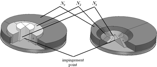
To address this question, the properties of the selected spatial trial functions should be discussed first. As already mentioned, the spatial functions were selected as functions of compact support. The description of such functions involves the definition of the sub-domains where they do not vanish. In the problem at hand, three zones have been defined. The first two are limited by coaxial circles with the centre at the impingement point. The third zone is the remaining portion of the surface of the piston.
When retrieving the heat flux, both linear and constant in space functions have been used. The first set of functions denoted by Con, consists of constant trial function in space for each zone. The second set denoted as Lin (), prescribes linear trial functions in the first and second zone.
This set the trial functions depend linearly on the distance from the central impingement point A. The variation of the HTC in the third zone is expected to be low. That is why a constant trial function is used in the outer zone. Associated with both sets of spatial functions are constant in time trial functions.
To retrieve temperature, one set of the trial functions was used. Those functions were constant in space but for the reasons already explained, linearly varying in time.
7. Mean HTC
As the heat flux is retrieved using constant in time trial functions, the mean value of the heat flux in Equation (30) is obvious. The retrieved temporal variation of the temperature in a zone is linear. It starts from known initial temperature T0 reaching z–the final temperature in this zone at the end of the experiment. The average temperature in a zone is determined from
(31)
and the HTC is evaluated as
(32)
Although the HTC is not estimated directly, the obtained results show that the accuracy and stability of the developed method is good.
8. Inverse analysis based on simulated experiments
Several tests were performed to validate the method. The approach used here was the pseudo-measurement technique where the results of the measurements were substituted by solution of a direct problem. The presence of measurement errors has been accounted for by adding random numbers of prescribed amplitude A. Random numbers were generated by RNUNF–internal Fortran ISML routine Citation12. This routine generates uniformly distributed numbers between 0 and 1.
A most conservative (pessimistic) approach of simulating the measurement error was applied. The amplitude of the error was always taken to be equal to A. Depending on the generated random number, this value has been either added to the simulated measurements (random number greater than 0.5) or subtracted from the pseudo-measurement.
Both the pseudo-measurements and the values of the auxiliary temperature fields were evaluated numerically using MSC.Marc, a commercial FEM package. To avoid the inverse crime Citation16,Citation17 different grid density depicted in were used in the inverse analysis and the direct problems used to generate the pseudo-measurement. The total number of tetrahedral elements in the inverse analysis runs was 51k while in the second 85k elements were used. Moreover, the pseudo-measurements have been simulated by assuming that the distribution of the HTC is described by a fifth-order polynomial and retrieved by a linear or constant spline.
Both heat flux and the HTC distributions were reconstructed and compared with the data used to simulate the measurements. The geometry, material properties, mesh and the trial functions used for validation purposes were identical with those used for genuine inverse analysis. The validation procedure was based on simulated time-to-arrival approach. The heat flux as well as the HTC was retrieved using both previously defined sets of trial functions: Con and Lin.
The time-to-arrival technique offers a possibility of treating each pixel of the registered bitmap as a temperature sensor. This feature was imitated by treating each FEM node located on ΓR surface as a pseudo-sensor. For the applied grid resolution, this produced a set of 1874 equations for determining the distribution of heat flux or HTC.
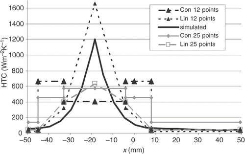
Test runs showed a strong dependence of the inverse analysis results on the number of sensors, especially in the central or intermediate zone. This sensitivity can be explained by the fact that each sensor yields only one information, i.e. its activation time. This is in contrast to the standard measurement technique, where a sensor can generate an arbitrary number of temperature readings. The attempt to obtain the results for 12 or 25 measuring points () distributed uniformly along the radius failed in all zones. The results show that the obtained values strongly depend not only on the number of the sensors but also on their location. Only a large number of sensors (case dependent) leads to stable results of the inverse analysis.
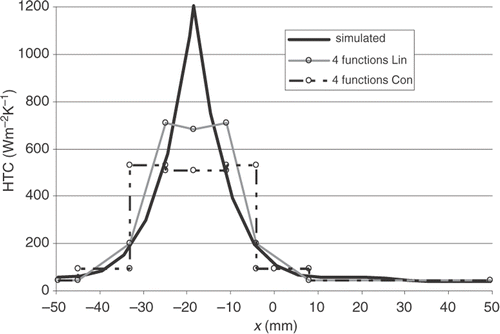
The most important values of the retrieved parameters are those in the central zone, near the impingement point, as there the HTC assumes the greatest values. To enhance the accuracy, this zone was subdivided into two subzones (A and B). Contrary to expectations, this approached led to instable results (). The reason for this is the small number of pseudo sensors in subzone A. The rapid warming up of the vicinity of the impingement point, causes all measurements concerning this zone to occur within a very short time interval, after which, all points of the subzone exceed the activation temperature. Thus no information about the variation of the temperature in the central subzone is available after a very short time.
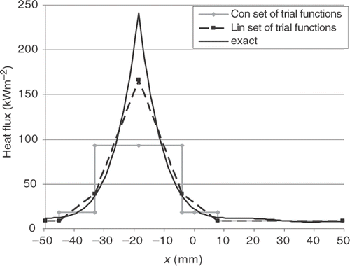
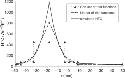
Intensive tests of the inverse analysis revealed that the stability of the procedure depends strongly on the number of applied (pseudo) sensors. Best results were obtained when all 1874 FEM nodes located on the upper surface of the probe were treated as pseudo sensors. The quality of the results both in the case of heat flux () and HTC reconstruction () was good with the exception of the peak value where the retrieved value is lower by about 30%. Results obtained using simulated error amplitude equal to 0 s, 0.5 s, 1s and 2 s are nearly identical (cf ), confirming the stability of the applied method. For the sake of clarity, and show only results corresponding to 0 error.
Table 1. Influence of measurement errors on retrieved flux and HTC. Simulated experiment.
9. Inverse analysis based on physical experiments
Seven measurement series were performed for different mass rates of the oil. Due to space limitations, only three sets are analysed in more detail: M7 with the highest oil flow rate, M2 with lowest and M4 with intermediate flow rate. The increase of the mass flow of oil causes the increase of the HTC and decrease of the measured activation time. Obviously, the first point to reach the activation temperature is the location opposite the centre of the impingement jet. As the distance between a given point and the impingement point increases, the activation time grows.
For the test with the maximum oil flow rate (M7), the activation time was between 2 s and 13 s while for the low oil flow rate (M2) the activation temperature was reached between 55 s and 113 s.
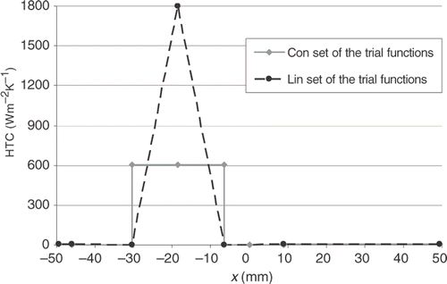
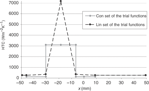
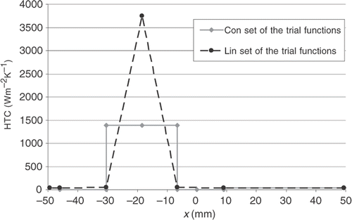
Inverse analysis employing both the already mentioned sets of trial functions yield for experiments M2, M7, M4 a distribution of the HTC shown in Figures .
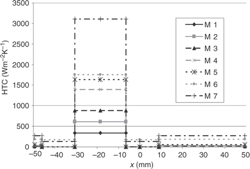
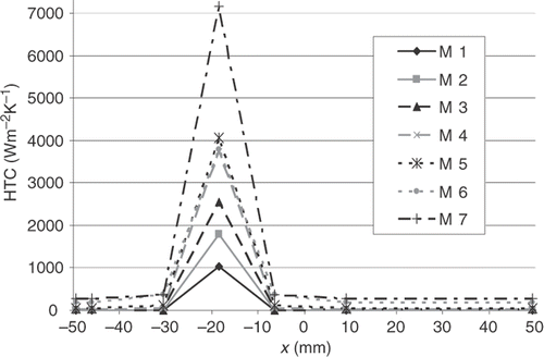
It can be seen that for experiment M2, the maximum value of the HTC at the impingement point obtained for the Lin set of functions is about 1800 W m−2K−1 while for Con set of trial functions it is only around 600 W m−2K−1. For both sets the HTC is equal to 0 in the second and third zone as confirmed by the experiments. The oil hit the surface at the impinged point, slid along the surface and dropped down approximately 10 mm away from the impingement point.
For experiment M7 the maximum value of the HTC obtained for the Lin trial functions was 7200 W m−2K−1, while for Con functions the retrieved value is about 3200 W m−2K−1. As expected the quality of linear approximation of HTC is better that its stepwise counterpart. Con set produced a non-physical value for the intermediate zone yielding a lower HTC value than in the outer zone.
Experiment M4 produces the maximum value of the HTC at the impingement point at the level of 3800 W m−2K−1 for linear trial functions and 1450 W m−2K−1 for constant.
To assess the quality of the obtained HTC distribution, the results of each series were verified by performing by a forward run of MSC.Marc using the retrieved values of the BC. The resulting temperatures corresponding to the experimentally determined times to arrivals were compared with the activation temperature. The error defined as
(33)
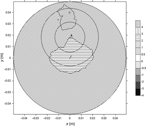
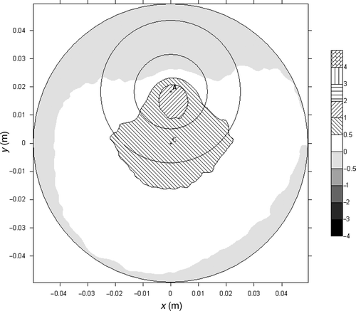
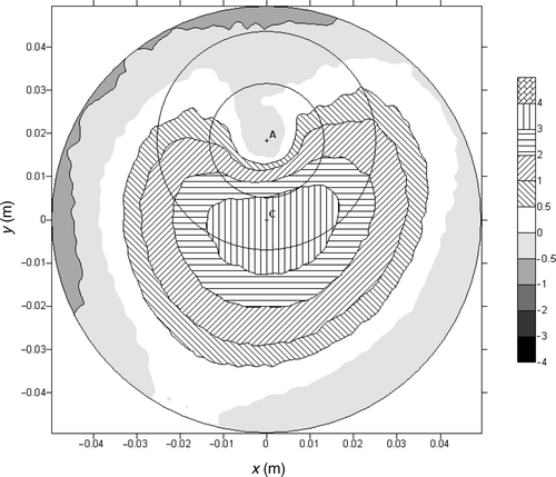
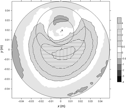
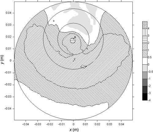
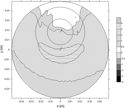
where Ts is the temperature obtained from the forward run using the retrieved HTC distributions, ta stands for time to arrival at a given point and Ta denotes the activation temperature. and show the error corresponding to experiment M7 for the Con and Lin set of trial functions. and depict the same values for experiment M2 while and for experiments M4. It can be seen that in experiment M2 the errors for the Lin set are significantly smaller than for their Con counterpart. For a large part of the boundary surface, the error is lower than 0.5 K, while for the constant functions it is between 1 and 2 K.
The errors corresponding to experiment M7 ( and ), are very similar. For the central zone for both sets errors are small and not exceed 0.5 K. For the intermediate zone errors for both sets vary in a range of 0–3.5 K.
The retrieved HTC distributions for all seven experiments are shown in and . As expected, the increasing oil flow rate results in enhanced heat transfer. It is obvious that the results obtained for the first set of the functions (Con) are less accurate than for the second one. Using constant trial functions (Con) the values of the HTC obtained for the intermediate zone, are for all cases, lower than for outer zone. This feature has no physical justification. The explanation might be that the values obtained for the central zone and outer zone are higher than in the reality. The fitting procedure lowers therefore the value obtained for intermediate zone. That kind of problem does not appear when linear functions are used. The results obtained in experiment M6 using the Lin set of trial functions are peculiar. The peak value is lower than for M5 series, corresponding to lower oil mass flow rate. Such a behaviour has no physical explanation. The only feasible explanation is a measurement error committed in this experiment. It should be stressed that the values in intermediate zone and outer zone are plausible.
10. Conclusions
The developed method is a general purpose inverse analysis technique for retrieving boundary temperature, heat flux and HTC. The central assumption of this approach is the linearity of the underlying direct problem, which allows us to resort to the superposition principle. As a result, the approach requires only a few solutions of the direct problems. The byproducts of the proposed approximation of the temperature field are the smoothed sensitivity coefficients obtained directly by solving a set of appropriately defined direct problems.
The next important feature of the proposed approach is that the retrieved function is approximated by a linear combination of locally based trial functions. These functions are analogue to the shape functions used in FEM but defined on a much coarser mesh.
The proposed approach is applicable to both steady state and transient problems. It is adapted to a specific measurement technique known as time-to-arrival. The developed inverse technique is accurate and stable, which has been proved by solving some simulated measurements problems.
The time-to-arrival approach makes the problem of the stability more pronounced. This may be explained by the fact that this technique yields a limited set of data (one information for each pixel). Therefore care should be exercised when deciding about the number of retrieved parameters. The attempt to estimate too many of them may significantly reduce the stability. Therefore finding the best possible solution is a matter of compromise between the number of degrees of freedom and the robustness of the algorithm.
Inverse analysis aiming at retrieving HTC distribution is more cumbersome than in the case of estimating temperatures and heat fluxes. While the latter two lead to linear inverse problems, retrieving HTC produces strong non-linearities even if the underlying direct problem is linear. The reason for this is the non-linear dependence of the temperature on the retrieved HTC. The developed technique proposes a way of circumventing this difficulty. The approach requires a solution of two linear inverse problems: for the heat flux and for the temperature. Once they are solved the HTC can be determined by resorting to the definition of the BC of Robin's type. This technique requires only a few solutions of linear boundary problems. The advantage of the developed method is that the direct solvers can be invoked before the iterative least squares loop is entered.
The obtained results show that the proposed approach is accurate and stable if only some precautions are taken. The main point here is to limit the number of the estimated degrees of freedom to the necessary minimum. The main limitation of the developed method is an arbitrary selection of the location of nodes of trial functions used to approximate the retrieved BC. To minimize the influence of this issue, any available information concerning the shape of the retrieved function should be embedded in the approximation formula (4) or (12). If the retrieved function assumes a maximum at a given point, a node of the trial function should be located at this very point. The method can also be extended to tackle non-linear problems. If this is the case, the entire procedure has to be embedded into an external loop where the temperature field is corrected.
There is also a possibility of retrieving the HTC by a special definition of time-dependent trial functions for the first and second BC. It ensures that for each time moment, the definition of third BC is fulfilled Citation18.
Another possible extension of the method is to use linear trial functions for both time and space variables. Such a choice of functions should improve the quality of the approximation while retaining the desired property of filtration of higher frequencies errors. However, the test calculations of retrieving the Dirichlet conditions using the time-to-arrival approach, do not produce satisfactory results. The same concerns other sets of the trial functions and subdivision of the central zone into two sub-zones. The explanation for it is the very short time needed to reach the characteristic temperature in the vicinity of the impingement point. After this short time has passed, there is no information about the process in this zone. Assuming linear variation of the temperature in time leads in such a case to extrapolation. The solution is extended far above the short temporal interval in which results of the measurements are available. Due to rapidly changing curvature of the temperature variation in time, the extrapolation produces unrealistic values. In this context, the assumption of constant time variation of the temperature stabilizes the solution, and produces more reliable results. To retrieve a higher order time variation, it is necessary to switch to the standard measurement technique of tracing the entire temporal variation of the temperature.
References
- Son, C, Gillespie, D, Ireland, P, and Dailey, GM, 2001. Heat transfer and flow characteristics of an engine representative impingement cooling system, J. Turbomachinery 123 (2001), pp. 154–160.
- Stevens, J, and Webb, BW, 1991. Local heat transfer coefficients under an axisymmetric, single-phase liquid jet, J. Heat Transfer 113 (1991), pp. 71–78.
- Elison, B, and Webb, BW, 1994. Local heat transfer to impinging liquid jets in the initially laminar, transitional, and turbulent regimes, Int. J. Heat Mass Transfer 37 (1994), pp. 1207–1216.
- Nada, SA, 2006. Slot/slots air jet impinging cooling of a cylinder for different jets–cylinder Configurations, Heat Mass Transfer 43 (2006), pp. 135–148.
- Han, J-C, 2004. Recent Studies in Turbine Blade Cooling, Int. J. Rotating Machinery 10 (2004), pp. 443–457.
- Souris, N, Liakos, H, and Fonti, M, 2004. Impinging jet cooling on concave surfaces, AIChE Journal 50 (2004), pp. 1672–1683.
- Yang, Y-T, and Tsai, S-Y, 2007. Numerical study of transient conjugate heat transfer of a turbulent impinging jet, Int. J. Heat Mass Transfer 50 (2007), pp. 799–807.
- Sharif, MAR, and Banerjee, A, 2008. Numerical analysis of heat transfer due to confined slot jet impingement on a moving plate, Appl. Thermal Eng 29 (2008), pp. 532–540.
- Jia, R, and Rokni, M, 2001. Impingement cooling in a rib-roughened channel with cross-flow, Int. J. Num. Meth. Heat Fluid Flow 11 (2001), pp. 642–662.
- Angioletti, M, Nino, E, and Ruocco, G, 2005. CFD turbulent modelling of jet impingement and its validation by particle image velocimetry and mass transfer measurements, Int. J. Thermal Sci. 44 (2005), pp. 349–356.
- Xu, F, and Gadala, MS, 2006. Heat transfer behavior in the impingement zone under circular water jet, Int. J. Heat Mass Transfer 49 (2006), pp. 3785–3799.
- "Visual Numerics: Fortran Subroutines for Mathematical Applications". Math library; pp. 958–964.
- Kurpisz, K, and Nowak, AJ, 1995. Inverse Thermal Problems. Southampton: Computational Mechanics Publications; 1995.
- Facchini, B, and Surace, M, 2006. Impingement cooling for modern combustors: Experimental analysis of heat transfer and effectiveness, Exp. Fluid 40 (2006), pp. 601–611.
- Białecki, RA, Divo, E, Kassab, AJ, and Ait Maalem Lahcen, R, 2003. Explicit calculation of smoothed sensitivity coefficients for linear problems, Int. J. Num. Meth. Eng 57 (2003), pp. 143–167.
- Wirgin, A, The inverse crime, Available at: arxiv.org/pdf/math-ph/0401050.
- Fadale, TD, Nenarokomov, AV, and Emery, AF, 1995. Uncertainties in parameter estimation: the inverse problem, Int. J. Heat Mass Transfer 38 (3) (1995), pp. 511–518.
- Ryfa, A, and Białecki, RA, Retrieving heat transfer coefficients by enforcing constant in time heat transfer coefficient, (in preparation).
