A simple method for inverse estimation of surface temperature distribution on a flat plate

Abstract

In this article, the temperature distribution of one surface of a flat plate is obtained from the solution of the inverse heat conduction problem (IHCP) based on the temperature measurement at the opposite surface of the plate. The modified one-dimensional correction method (MODCM), along with the finite volume method, is employed for both the two- and three-dimensional inverse problems. A series of numerical experiments are conducted in order to verify the effectiveness of the method. In addition, the effect of the factors, such as the temperature measurement error and the thermal conductivity of the flat plate, on the identification results of the temperature distribution is also studied. It is demonstrated by the numerical experiments that the method is a simple, stable and accurate one for this IHCP. The identification results are not sensitive to the measurement error of the inspection surface.

Keywords:

• inverse heat conduction problem
• modified one-dimensional correction method
• temperature distribution
• finite volume method

1. Introduction

It is always necessary to estimate the surface conditions, such as temperature and heat flux, accurately in the fields related to thermal engineering. However, one may encounter difficulties in directly measuring these parameters in many industrial applications such as the re-entry of a space vehicle and the nuclear reactor at loss of coolant event. A clue to solving this problem is to estimate these desired parameters based on the indirect temperature measurement according to the method of inverse heat conduction problem (IHCP).

Many methods have been developed for the inverse boundary condition estimation problem. Based on the recurrent neural networks, Lecoeuche et al. 1 successfully estimated the heat flux applied on one side of a structure from the knowledge of the temperature measured at the other side of the structure. The conjugate gradient method was also used by Huang and Chen 2, Huang and Wang 3, Loulou and Scott 4, Groß et al. 5 and Yang et al. 6 for the determination of the steady or time-dependent heat flux distribution. In their work, the conjugate gradient method was used to update the heat flux estimation until the convergence of the calculated and the measured temperature distributions. The Levenberg–Marquardt method was also used by Su et al. 7 for the estimation of the spatially non-uniform wall heat flux in turbulent circular pipe flow.

For the heat transfer coefficient estimation, Osman and Beck 8 treated the problem of estimating the time-dependent heat transfer coefficient in quenching a sphere as a non-linear parameter estimation problem. Xu and Chen 9 studied the non-linear problem of determining the heat transfer coefficient in two-phase mixture flow in an inclined tube by building a steady-state two-dimensional heat conduction model. Martin and Dulikravich 10 developed an inverse boundary element method procedure for the determination of the unknown heat transfer coefficients on surfaces of arbitrarily shaped solids. The procedure is non-iterative and cost effective. Chantasiriwan 11 also presented an algorithm for the estimation of the time-dependent heat transfer coefficient for one-dimensional linear IHCP based on the sequential function specification method with the assumption of linearly varying future boundary heat flux components.

As to the estimation of temperature distribution, Monde et al. 12 developed an analytical method based on the Laplace transform technique to determine the surface temperature and heat flux. Chen et al. 13 presented a hybrid numerical algorithm of the Laplace transform technique and finite difference method with a sequential-in-time concept and the least-square scheme to predict the unknown surface temperature in two-dimensional IHCP. Wu and Chu 14 applied the space-marching technique to the estimation of the temperature distributions and unknown boundary conditions from internal measurements. A gradient-based inverse method combined with B-spline function specification was employed by Kim and Lee 15 to solve the inverse problem on determining the steady-state unknown surface temperature distribution. The validity of the proposed method was verified with computational results.

In this article, a simple numerical method is presented for estimating the temperature distribution for a multidimensional IHCP. The method used is the modified one-dimensional correction method (MODCM) which is a simple but accurate inverse method that can deal with the multidimensional IHCP by using a one-dimensional inverse function. The discrepancy of the estimated results caused by the one-dimensional simplification is then corrected during the iteration process. Recent results by Fan et al. 16–18 showed that this method yielded good estimates of the inner pipe boundary shape, the distribution of the effective thermal conductivity of the interlayer of a sandwich plate and the interfacial geometry of a multiple region domain based on the surface temperature measurement. Hence it is expected that the identification of temperature distribution should perform well with the method as well, especially for the three-dimensional inverse problem. Meanwhile, the effect of the random measurement error and the thermal conductivity of the test piece will also be discussed.

2. Mathematical formulation of the problem (direct problem)

The problem to be considered is shown schematically in Figure 1. The temperature distribution on the left surface of the plate is to be determined. From the inspection surface, i.e. the right surface, heat is dissipated to ambient by convection with a constant film coefficient h_n. The other four surfaces of the test piece are insulated. The temperature distribution at the inspection surface is measured by an infrared imager or thermocouples. The ambient temperature is T_a. The size of the flat plate is described by L_x, L_y and L_z in x, y and z directions, respectively. The measured temperature data along with the known geometrical and thermophysical data give rise to the IHCP, which can be mathematically described by the following steady-state governing equation and boundary conditions for the whole plate: (1) Boundary conditions: (2) (3) (4) (5)

Figure 1. The three-dimensional inverse problem to be solved for the temperature distribution T_l(x,y).

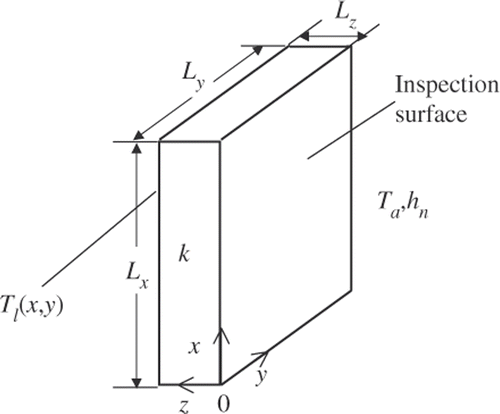
In the inverse problem, all parameters illustrated in Figure 1 are known except the temperature distribution T_l(x,y) of the left surface. The goal of the IHCP solution is to determine the temperature distribution T_l(x,y) based on the temperature measurements of the inspection surface.

3. The MODCM (inverse problem)

3.1. Introduction of the MODCM

The MODCM is developed in our previous work 16–18 on the basis of the one-dimensional correction method (ODCM) presented by Yang et al. 19 by correcting the iteration function, modifying the calculation of the correction criterion and giving the stopping criterion of the iteration. In 16–18, the MODCM showed good performance in solving the inverse problems on the identification of boundary geometry and conductivity distribution.

The MODCM first calculates the parameters to be determined for the multidimensional inverse problem based on a one-dimensional inverse function. Then the discrepancy caused by the one-dimensional simplification is corrected by iteration. The expression of the iteration function is developed based on Taylor's series expansion.

For the inverse problem of concern in this article, the temperature distribution T_l(x,y) is described by a matrix formed by the discrete temperature value T_li,j (i = 1∼m_x; < br/ > j = 1∼m_y) where m_x and m_y are the numbers of the node layers in x and y directions, respectively. The term T_li,j is first calculated based on the corresponding discrete temperature measurements T_oi,j(i = 1∼m_x;j = 1∼m_y) of the inspection surface, i.e. the element of the measured temperature matrix , according to the one-dimensional inverse function T_l1D(T_o) which can be deduced easily from the one-dimensional heat conduction problem.

The Taylor's series expansion at an arbitrary temperature is (6) Then for the problem of concern in this article, the temperature distribution of the left surface T_li,j(T_oi,j) can be updated on the basis of the initial estimation T_li,j(T_i,j), where T_i,j is the temperature distribution of the inspection surface calculated according to the multidimensional equation (1) based on the initial estimation of the temperature distribution of the left surface, for each discrete point by (7) where the subscript o denotes the original temperature measurement of the inspection surface. Of course, the precise estimation cannot be obtained by using Equation (4) once. Then a corrective function can be derived based on Equation (4) for refining T_li,j(T_oi,j) of an arbitrary discrete point of the left surface: (8) where and are determined for each iteration through numerical calculations and the superscript n is the iteration number. The term is the difference between the measured temperature data of the inspection surface and the calculated temperature of the inspection surface according to the multidimensional equation (1) based on the estimated temperature distribution of the left surface of the n-th iteration.

When the parameters in Equation (5) are written in matrixes, the iteration process can then be described as (9) If the last term is neglected, Equation (6) becomes (10) where is the n-th estimate of the temperature distribution of the left surface after n − 1 iterations; is a matrix formed by the element which describes the temperature distribution at the inspection surface when the temperature distribution of the left surface is ; is the original measured temperature distribution at the inspection surface; and are the correction terms; the symbol ‘*’ in Equations (6) and (7) denotes the Hadamard product, i.e. the element by element product, of two matrixes with the same size and the superscript n is the iteration number. It should be mentioned that, in Equations (6) and (7), the matrixes , , , and have the same size m_x × m_y. It seems that the temperature distribution of the left surface is updated point by point separately, but actually all the discrete points are correlated during the iterative process when calculating the correction terms and .

3.2. Obtaining correction criterion

As in 19, the two terms and can be determined after each iteration based on (11) The term in Equation (8) of each iteration can be computed, according to 18, by perturbing the element T_li,j of the vector obtained from the last iteration one-by-one and computing the resulting change in temperature T_i,j of the corresponding point of the inspection surface from the solution of the multidimensional heat conduction problem in Equation (1). Thereafter, is calculated by the ratio of perturbations of the two parameters: δT_i,j/δT_li,j. Then the two terms and can be obtained to get and according to Equation (8).

3.3. Stopping criterion of the iteration

The stopping criterion of the iteration of the MODCM for the identification of the temperature distribution is given as (12) where ϵ is a small positive number; m_x and m_y represent the numbers of the node layers in x and y directions, respectively, and the superscript n denotes the iteration number. When the random temperature measurement error is in consideration, the discrepancy principle 20 is adopted in this article: (13) where σ is the standard deviation of the temperature measurements.

3.4. Computational procedure of the MODCM

The iterative computational procedure for the solution of this temperature distribution identification problem using the MODCM can be summarized as follows:

Compute the initial temperature distribution based on the measured temperature distribution at the inspection surface by using the one-dimensional inverse function T_l1D(T_o) to begin the iteration process. Suppose is available after n − 1 iterations.

1.	Compute the temperature distribution at the inspection surface based on the estimated temperature distribution of the left surface according to the multidimensional heat transfer problem in Equation (1) by the finite volume method.
2.	Check the stopping criterion given by Equation (9), go on if not satisfied.
3.	Compute the correction terms and based on the estimate of the temperature distribution by the perturbation method in Section 3.2.
4.	Calculate the new temperature distribution based on Equations (6) or (7), then return to Step (1). In this article Equation (7) is used.

4. Numerical experiments and discussion

To illustrate the validity of the present inverse algorithm in identifying the temperature distribution T_l(x,y) of the left surface of the flat plate test piece in Figure 1 from the knowledge of temperature recordings at the inspection surface, we consider a series of numerical examples, two-dimensional and three-dimensional, in this section with different temperature distributions.

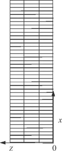
In all test cases considered here, we have chosen T_a = 25°C and h_n = 10 Wm⁻² K⁻¹. Equation (1) is solved by the finite volume method. The number of node layers of the flat plate in z direction is 4. For the two-dimensional study, the number m_x of the node layers in x direction is set as 41, which is shown schematically in Figure 2; while for the three-dimensional one the numbers in both x and y directions are 21, namely m_x = 21 and m_y = 21. These node numbers are selected based on the numerical grid-independent tests. As in many studies of the IHCPs 3,20, in the numerical experiments the measured temperature distribution at the inspection surface is simulated by the solution of the multidimensional equation (1) calculated based on the known temperature distribution of the left surface, and to which errors can also be added to simulate real temperature measurements. The simulated inexact measurement data can be expressed as (14) where is the solution of Equation (1) along with the boundary conditions in Equation (2) based on the known exact temperature distributions to be determined; σ is the standard deviation of the measurement and is a vector with the same size as formed by random numbers between −1.0 and 1.0. Based on these simulated temperature measurements the identification work is conducted and the results will be compared with the known exact temperature distributions to verify the effectiveness of the algorithm.

Figure 2. Schematic of grid meshing of the plate for two-dimensional test cases.

In order to describe the precision level of the identification results, an average relative error (ARE) is defined by comparing the estimated and the exact (known) temperature distributions of the left surface as (15) where T_li,j is the estimated result; denotes the known temperature distribution of the left plate surface.

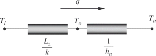
The one-dimensional inverse function T_l1D(T_o), which will be used to calculate the initial temperature distribution, can be derived easily based on the measured temperature T_o of the inspection surface according to the thermal resistance distribution in the one-dimensional heat transfer problem shown in Figure 3 as (16) where k is the thermal conductivity of the flat plate.

Figure 3. Thermal resistance distribution of the one-dimensional heat transfer problem of the plate.

4.1. Two-dimensional numerical test cases

If the dimension of the flat plate in y direction is very long relative to the ones in z and x directions and the temperature distribution of the left surface of the plate does not change in y direction either, the IHCP on determining the temperature distribution can be deemed as of two dimension.

For this two-dimensional problem, the dimensions of the test piece are adopted as L_z = 0.1 m and L_x = 0.5 m. The functions of the temperature changing in x direction of the two test cases are as follows: (17) (18)

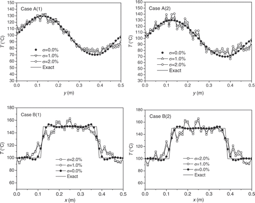
In order to study the effect of the thermal conductivity of the test piece on the estimation of the temperature distribution, two thermal conductivities are adopted: one is 30.0 Wm⁻¹ K⁻¹, and the other is 0.1 Wm⁻¹ K⁻¹. The numerical examples corresponding to these two conductivities are denoted by Case A(1), Case B(1) and Case A(2), Case B(2), respectively. Based on Equation (1) the temperature distributions at the inspection surface are calculated numerically by the finite volume method and plotted in Figure 4. Based on these temperature distribution curves, i.e. the simulated temperature measurements, the identification work is conducted to certify the effectiveness of the inverse method.

Figure 4. Temperature distributions at the inspection surface for test Case A and Case B.

When no measurement error is considered (σ = 0), the identification results of the temperature distribution of the left plate surface are shown in Figure 5 when the stopping criterion is set as ϵ = 0.001 which is selected based on the beforehand tests. The ‘exact’ curves in the figures are plotted based on the known temperature distributions described in Equations (13) and (14). The AREs of the identification results are reported in Table 1. From both the figures and the table, one can see that the estimated and the exact curves have a good agreement. Though the AREs of test cases B(1) and B(2) are relatively larger, the largest value is still less than 5%. In the figures, the initial identification results of the temperature distributions are also shown which were obtained only by using the one-dimensional inverse function (12) before the iteration begins. These ‘initial’ curves tell us that one-dimensional simplification will cause an obvious discrepancy in the identification results; therefore the iterative correcting process is necessary.

Figure 5. Identification results of the temperature distributions when no measurement error is considered for Case A and Case B (ϵ = 0.001).

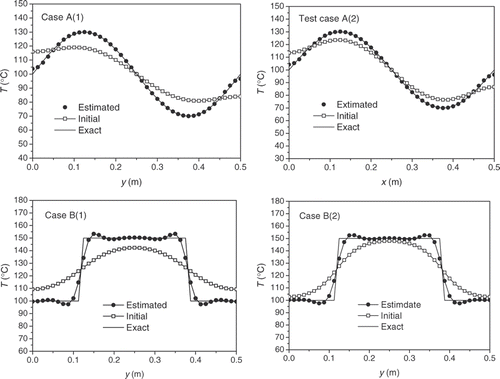
Table 1. Relationship between the measurement error and the ARE of identification results.

	ARE (%)
σ (%)	Case A(1)	Case A(2)	Case B(1)	Case B(2)
0.0	0.37	0.43	2.1	2.2
1.0	3.8	4.8	6.2	6.1
2.0	5.4	8.2	7.0	7.5

When the random errors of the temperature measurement are added to the exact temperature distribution, a temperature curve with sharp changes is obtained. For the heat transfer in the plate has the ‘smooth’ character, the temperature distribution with sharp changes of the inspection surface is impossible to obtain no matter what the temperature distribution of the left surface is; therefore it is meaningless to expect the stopping criterion in Equation (9a) to be zero. In this article, the stopping criterion based on the discrepancy principle, which is related to the standard deviation of temperature measurement and also to the discrete point number, is introduced in the MODCM to measure the acceptable convergence between the calculated and the measured temperature distributions. The identification results for the two test cases are shown in Figure 6. In this article, the standard deviation of the temperature measurement is described by the percentage of the average temperature of the inspection surface. The AREs of the identification results are also listed in Table 1. The largest ARE is less than 8.2% when the standard deviation of temperature measurement is not more than 2.0%. Confident results can be accepted as the solution of the inverse problem. For the plate with smaller conductivity, it is easier to obtain a zigzag temperature distribution of the inspection surface; therefore, more accurate results can be obtained based on Equation (9b) for the plate with larger conductivity.

Figure 6. Identification results of temperature distributions when random measurement error is considered.

4.2. Three-dimensional numerical test cases

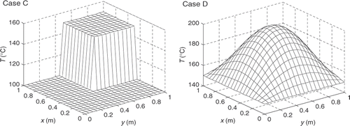
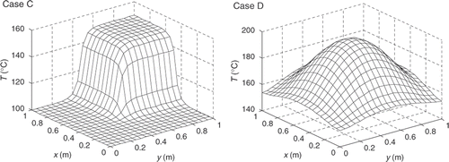
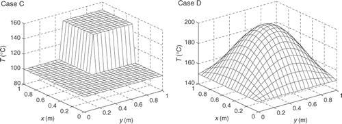
In this subsection, the numerical method is tested for solving the three-dimensional IHCP for determining the temperature distribution of the left surface of the plate shown in Figure 1. The dimensions of the plate tested are L_x = 1.0 m, L_y = 1.0 m and L_z = 0.1 m. The temperature distributions to be determined are shown in Figure 7. The thermal conductivities of the plate are 0.1 and 30.0 Wm⁻¹ K⁻¹ for Cases C and D, respectively. Based on the simulated temperature distributions at the inspection surface which are obtained according to Equation (1), the temperature distributions are estimated first based on the one-dimensional inverse function (12) and plotted in Figure 8. Then the discrepancy caused by using this one-dimensional inverse function is corrected by the iteration process according to Equation (7). The final identification results of the temperature distributions are shown in Figure 9 when the stopping criterion is adopted as ϵ = 0.001. The AREs of the results for Case C and Case D are 0.02 and 0.009%, respectively, when no measurement error is considered. The estimated and the exact temperature distributions have a very good agreement.

Figure 7. Exact temperature distributions to be determined for Case C and Case D.

Figure 8. Initial identification results of temperature distributions according to function (12).

Figure 9. Final identification results of temperature distributions for Case C and Case D (ϵ = 0.001).

When the random error of the temperature measurement is considered, the identification results of the test Cases C and D are plotted in Figures 10 and 11. The AREs of more numerical examples are reported in Table 2. From both the figures and the table, one can see that confident identification results can still be obtained when random error is considered and that the identification results are not sensitive to the measurement error since the largest ARE is not more than 12.0% when σ is less than 5.0% of the average temperature of the inspection surface.

Figure 10. Identification results of temperature distributions for Case C and Case D with random measurement error in consideration (σ = 1.0%).

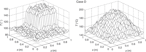
Figure 11. Identification results of temperature distributions for Case C and Case D with random measurement error in consideration (σ = 2.0%).

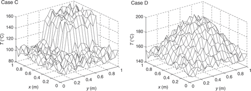
Table 2. Relationship between the ARE and the standard deviation of the measurement.

σ (%)	ARE (Case C) (%)	ARE (Case D) (%)
0.0	0.02	0.009
0.5	1.9	0.9
1.0	2.8	1.5
2.0	5.0	2.0
5.0	12.0	4.7

From the preceding two- and three-dimensional test cases, it is concluded that the MODCM is now applied successfully in this multidimensional inverse heat conduction problem for predicting the unknown steady temperature distribution. It should also be mentioned that the present method is very fast: all the results in this article are obtained within 3.0 min.

5. Effect of discrepancy principle in MODCM

As discussed in 19 when the ODCM was first presented, because the numerical method used in the MODCM is one of those for regular problems of differential equations, the errors which occurred in practical temperature measurement would only lead to errors in the identification results, but will not make the method itself ill-posed; therefore, stable solutions of the inverse problem can be obtained by using the MODCM even when no regularization measures are taken.

However, as shown in our previous work 17, when the stopping criterion of the iterative process is used in the following form, (19) the result of the method can be deemed as very precise but only for the new numerical case with temperature measurement error added; therefore, the errors resulting from the temperature measurement errors are included in the estimation results. This error is relatively difficult to determine as it varies with the value of the parameter to be estimated. But when the discrepancy principle is introduced in this article, the optimum solution, which makes the calculated temperature distribution match best to the measured, can be obtained; no estimation and elimination of the error in the estimation results are needed any more. This can be proved by the estimation results in the above numerical experiments which can be accepted directly as confident results of the inverse problem.

6. Conclusion

The MODCM was successfully applied for the solution of the IHCP to determine the unknown temperature distribution by utilizing the temperature readings at the inspection surface of a flat plate. Several test cases involving different functional forms of the unknown temperature distribution and different measurement errors were considered. The numerical testing results concluded that identification results with high accuracy can be obtained as long as the temperature measurement is precise and that the identification results are not sensitive to the random temperature measurement error. The discrepancy principle can guarantee the method to find the optimum result.

In comparison with other iterative regularization methods, the MODCM has the following advantages:

i.	Stable: The stability of the method can guarantee the convergence of the solution because the numerical method used in the algorithm is one of those for regular problem of differential equation.
ii.	No initial guess is needed: In many methods, the initial guess may have an obvious effect on the precision level of the identification results. In the MODCM, the initial value of the parameters is determined by the one-dimensional inverse function based on the temperature recordings on outer surface.
iii.	No matching problem is confronted: In most of the optimization methods used in the inverse problem, the desired parameters are refined by iteration until the temperature distribution computed is close to that measured. The problem of how to match the measured and calculated temperature values is difficult in practical work. But, in the MODCM, the distribution of the discrete points on the opposite boundary is determined according to the measurement point distribution on measuring surface when calculating the initial parameter value based on the inverse one-dimensional function, no matching problem exists.
iv.	Can estimate more complicated distribution of parameters because the MODCM almost updates the parameter of every discrete point separately. The discrete points are correlated only when calculating the correction terms during the iterative process.

This method is promising to be extended to solve other inverse problems. However, the MODCM is currently still restricted to solving the problem of estimating the unknown parameters on the opposite side of the temperature measurement; further theoretical study is yet to be done.

Acknowledgements

The author would like to acknowledge the financial support from the Natural Science Foundation of NUE, grant number HGDJJ05009.

References

- Lecoeuche, S, Mercere, G, and Lalot, S, 2006. Evaluating time-dependent heat fluxes using artificial neural networks, Inverse Prob. Sci. Eng. 14 (2006), pp. 97–109.
- Huang, CH, and Chen, WC, 2000. A three dimensional inverse forced convection problem in estimating surface heat flux by conjugate gradient method, Int. J. Heat Mass Transfer 43 (2000), pp. 3171–3181.
- Huang, CH, and Wang, SP, 1999. A three dimensional inverse heat conduction problem in estimating surface heat flux by conjugate gradient method, Int. J. Heat Mass Transfer 42 (1999), pp. 3387–3403.
- Loulou, T, and Scott, EP, 2003. Estimation of 3-dimensional heat flux from surface temperature measurements using an iterative regularization method, Heat Mass Transfer 39 (2003), pp. 435–443.
- Groß, S, Soemers, M, Mhamdi, A, Sibai, FA, Reusken, A, Marquardt, W, and Renz, U, 2005. Identification of boundary heat fluxes in a falling film experiment using high resolution temperature measurements, Int. J. Heat Mass Transfer 48 (2005), pp. 5549–5562.
- Yang, YC, Wu, TS, and Wei, EJ, 2007. Modeling of simultaneous estimating the laser heat flux and melted depth during laser processing by inverse methodology, Int. Commun. Heat Mass Transfer 34 (2007), pp. 440–447.
- Su, J, Lopes, AB, and Neto, AJS, 2000. Estimation of unknown wall heat flux in turbulent circular pipe flow, Int. Commun. Heat Mass Transfer 27 (2000), pp. 945–954.
- Osman, AM, and Beck, JV, 1990. Investigation of transient heat transfer coefficient in quenching experiments, ASME J. Heat Transfer 112 (1990), pp. 843–848.
- Xu, J, and Chen, T, 1998. A nonlinear solution of inverse heat conduction problem for obtaining the inner heat transfer coefficient, Heat Transfer Eng. 19 (1998), pp. 45–53.
- Martin, TJ, and Dulikravich, GS, 1998. Inverse determination of steady heat convection coefficient distributions, ASME J. Heat Transfer 120 (1998), pp. 328–334.
- Chantasiriwan, S, 2000. Inverse heat conduction problem of determining time-dependent heat transfer coefficient, Int. J. Heat Mass Transfer 42 (2000), pp. 4275–4285.
- Monde, M, Arima, H, and Mitsutake, Y, 2003. Estimation of surface temperature and heat flux using inverse solution for one-dimensional heat conduction, ASME J. Heat Transfer 125 (2003), pp. 213–223.
- Chen, HT, Lin, SY, and Fang, LC, 2001. Estimation of surface temperature in two-dimensional inverse heat conduction problems, Int. J. Heat Mass Transfer 44 (2001), pp. 1455–1463.
- Wu, SK, and Chu, HS, 2004. Inverse determination of surface temperature in thin-film/substrate systems with interface thermal resistance, Int. J. Heat Mass Transfer 47 (2004), pp. 3507–3515.
- Kim, SK, and Lee, WI, 2002. Inverse estimation of steady-state surface temperature on a three-dimensional body, Int. J. Numerical Meth. Heat Fluid Flow 12 (2002), pp. 1032–1050.
- Fan, C, Sun, F, and Yang, L, 2008. A new computational scheme on quantitative inner pipe boundary identification based on the estimation of effective thermal conductivity, J. Phys. D: Appl. Phys. 41 (2008), p. 205501.
- Fan, C, Sun, F, and Yang, L, 2008. A numerical method for determining thermal conductivity distribution of the interlayer of a sandwich plate based on thermographic temperature measurement, J. Phys. D: Appl. Phys. 41 (2008), p. 135501.
- Fan, C, Sun, F, and Yang, L, 2009. An algorithm study on inverse identification of interfacial configuration in a multiple region domain., ASME J. Heat Transfer 131 (2009), p. 021301.
- Yang, L, Geng, W, Jiang, L, Zou, L, and Hong, J, 1999. Profile identification in dynamic infrared thermography: Adaptability and stability, Int. J. Infrared Millimeter Waves 20 (1999), pp. 623–634.
- Ozisik, MN, and Orlande, HRB, 2000. Inverse Heat Transfer: Fundamentals and Applications. New York: Taylor & Francis; 2000.