Identifying an unknown source term in a heat equation

Abstract

We consider the problem of identifying an unknown source which depends on the spatial variable, in a heat equation. This is an ill-posed problem in the sense that the solution (if it exists) does not depend continuously on the data. To obtain a stable numerical solution, we propose an interesting regularization method based on the idea of quasi-reversibility method. The error estimate between the exact solution and its regularized approximation is given. We also discuss the numerical implementation and give several examples to verify the effectiveness of the proposed method.

Keywords:

• ill-posed problem
• unknown source
• regularization
• quasi-reversibility method

AMS Subject Classifications::

• 65M30
• 35R25
• 35R30

1. Introduction

Consider the problem of finding a pair of functions satisfying (1) where or , and in the latter case also the boundary conditions (2) is to be fulfilled.

In practical applications, the input data g can only be measured, so we actually have the measured data function which is merely in , and satisfies (3) where denotes L²-norm, and the constant δ > 0 represents the noisy level of input data.

This problem can be seen as a problem of source identification from measured data for the heat equation, which is important in many branches of engineering sciences. For example, an accurate estimation of pollutant source is crucial to environmental safeguard in cities with high populations. This problem has been investigated in many articles. To the author's knowledge the existence and uniqueness of the solution have been investigated in 1–3, the conditional stability and the data compatibility have been studied in 4–6, and the numerical algorithms for the identification problem can be found in 7–12. However, the general regularization analysis for the problem is still very limited. In 13, the regularization has been studied by the Fourier method, and error estimates have been given in the implicit representation.

In the present work, we make a new attempt, i.e. adding a perturbation term in the heat equation and considering the following equation instead: (4) This is based on the idea of the quasi-reversibility method, which was proposed by Lattès and Lions in 14. The idea of this method has been successfully used for solving various types of ill-posed problems, e.g. for sideways heat equation in 15,16, and backward heat conduction problem in 17. For the Cauchy problem of Laplace's equation, the authors refer to 18. In (4), the choice of α is based on some a priori knowledge about the exact solution f(x) and the measurement error bound (3). We give an error estimate in Section 3, which shows that this equation can be used to approximate the solution of (1). Our method is interesting because it can be discretized using standard techniques, e.g. finite differences (Section 4). Although in this article we mostly discuss the heat equation with source term in its simplest form , our interest is in numerical methods that can be used for more general problems which occur in applications, e.g. equations with non-constant coefficients, (5) non-linear problems (6) or source term has the representation , i.e. (7) where ϕ(t) is known and independent of the space variable x. This problem is related to determine the density of radioactive heat source by the thermal radiation on the surface, for example, if 6. For problem (7), we add the term at the right-hand side, then it can be analysed analogously to problem (1). For problems (5) and (6) one cannot use general methods reformulating the problems. Instead, we propose to add at the right-hand side, discretize these problems and solve them essentially in these discrete forms. The numerical aspect of our method can be implemented by the finite difference scheme and some examples given in Section 5 are used to verify the usefulness of our method.

2. Ill-posedness of problem (1) and regularization

The problem of source identification is ill-posed in the sense that the solution, if it exists, does not depend continuously on the data. In this article, we only consider the case that , the ill-posedness can be seen in the following discussion.

By separation of variables, we obtain that the solution of problem (1–2) has the form (8) where is an orthogonal basis in . We define the operator , then we have It is easy to see that K is a linear compact operator, and the singular values of K satisfy and i.e. Therefore, (9) Note that as , thus the exact data function g(x) must satisfy the property that (g, u_n) decay rapidly as . As for the measured data function , we cannot expect it to have the same decay rate in . Thus the problem is ill-posed 19, and some special regularization methods are required.

A convenient method for constructing classes of admissible regularization strategies is given by filtering singular systems, i.e. damp the factors by , where is a regularizing filter with the following properties 20:

1.	for all α > 0 and ;
2.	for every α > 0 there exists c(α) such that
3.	for every .

Thus the regularized solution is defined by We now list some regularizing filters of well-known regularization strategies for solving problem (1). Corresponding to the Tikhonov regularization strategy 19,20, the regularizing filter could be (10) where α_T is a small positive parameter.

Corresponding to the Landweber regularization strategy 19–21, the regularizing filter has the form (11) for some .

In addition, (12) (13) (14) are regularizing filters corresponding to three spectral methods 20,22, respectively, where α_s1, α_s2 and α_s3 are small positive parameters.

From (10–14) we conclude that, on the one hand, if the parameter α is small, is close to . It means that the smaller the parameter α, the closer the regularized solution f_α approximates to the exact solution f. On the other hand, if the parameter α is fixed, the regularized solution f_α will depend continuously on the data g. Actually, the bigger the parameter α is, the better the degree of regularized solution depending continuously on the data. Hence, we need a strategy to choose a proper parameter α in order to balance these two aspects. This conforms to the general regularization theory. The idea of using regularizing filters is very convenient and efficient for the purpose of theoretical analysis. For a more detailed explanation of this idea we refer to 23.

Now we introduce a new regularization method for problem (1) by adding a second derivative of the unknown source function in the equation. Let be the solution of following perturbed problem: (15) for small α > 0.

Similar to (9), we easily get (16) It can be seen that, (17) is a new regularizing filter and the regularization strategy we constructed is feasible. The regularizing filter in (17) has a simpler representation than (10–14). Moreover, system (15) can be easily discreted by standard techniques, e.g. finite differences. In this sense, our method can also be applied to problems with variable coefficients. This is actually a major advantage over other filters based on a sum of series formulation. In the following, we will take (16) as an approximation of the exact solution f(x).

We have not seen the problem (15) treated in the literature, and at present we are not deeply concerned with theoretical questions related to the problem (15). The main objective of this investigation is to find out how well (15) approximates (1) considered as a problem of source identification.

Since the convergence rates can only be given under a priori assumptions on the exact data 19, we will formulate such an a priori assumption in terms of the exact solution f(x) by considering (18) where denotes the norm in Sobolev space defined by: (19)

3. Error estimate

We now study the properties of (16) as an approximation to (9). The main conclusion of this article is given by the following theorem.

THEOREM 3.1

Let f given by (9) and given by (16) be the solutions of problem (1) and its perturbed problem (15), respectively. Suppose that conditions (3) and (18) hold. Then if the regularization parameter α is chosen as (20) there holds the error estimate (21) where .

Proof

Due to (9) and (16), we know (22) The assumptions (3) and (18) lead to (23) where (24) We start by estimating the second term on the right-hand side of (23). Since is monotonically decreasing with respect variable n, we have To estimate the first term on the right-hand side of (33), we will distinguish two cases.

Case I

For large values of n, i.e. for , we have (25)

Case II

For n < n₀, we have If 0 < p < 2, the above inequality becomes (26) else if p ≥ 2, we get (27) Combining (25–27), we obtain (28) Therefore, Since , and the ‘=’ obtains iff a = b, we set , i.e. we choose , and obtain the estimate (21).

Remark 3.2

Since the regularization parameter α→0 as the error bound δ→0, we can easily find that (29)

Remark 3.3

Since is usually unknown in applications, we have no exact a priori bound E. However, if we select , where c is a positive constant, there also holds (30) where the constant C depends upon . This choice of α is helpful in actual applications.

Note also that if we choose p = 0, i.e. the a priori assumption is replaced by , then there would only yield boundness of the terms in (21), (29) and (30) instead of convergence to zero 19.

Remark 3.4

For the case , we can obtain the solution by Fourier transform. And the analysis process analogous to will not to be described in detail.

4. Numerical tests

The numerical results presented in this section for the inverse source problem indicate that the proposed method is feasible and efficient. The tests were performed in the following ways: first we selected a solution f(x), , by solving a well-posed problem for the heat equation using a finite difference scheme to obtain the data , then we added a random distributed perturbation to the data and obtained the noisy data , i.e. (31) where ’ is a normally distributed random variable with zero mean and unit standard deviation and ϵ dictates the level of noise. Denote be partitions of the interval , and be the step length on space coordinates. The total noise level δ can be measured in the sense of Root Mean Square Error (RMSE) according to (32) Finally we solve problem (15) using as data by finite difference based upon the Crank–Nicolson method, and obtain the computed approximation . Then we compare the computed approximation with the exact solution.

In the following, we first give an example which has the exact expression of the solution u(x, t).

Example 1

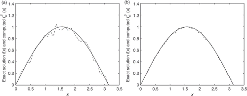
It is easy to verify that the pair of functions (33) is the exact solution of problem (1) with data (34) We will give the comparison of the exact solution and the computed approximation for perturbations and in Figure 1. We choose the step length k of x-variable as , the a priori bound E = 1 and p = 3/2. Then δ is given by (32), and α is chosen by (20).

Figure 1 shows that the proposed approach seems to be useful and the smaller the error is, the better the result will be. But in order to more distinctly show the serviceability and limitation of our method we give some tables.

In Tables 1–3, we select p = 2, E = 1 and α according to (26). The errors of the recovered f(x) are measured by the relative weighted l²-norm given by (35) In Table 4, we choose the step length , the perturbation , p = 3/2, E = 1, and δ is given as in (32), .

From Tables 1–3, we find that for a different choice of the step length in variables x and t, the differences of the regularization results are tiny. The method works well for a small perturbation error, and the smaller the perturbation error is, the better the result will be. However, for problems with higher error levels (e.g. ε = 10^-1), the results are less encouraging. It is well known that the discretization of x-derivative induces regularization 24, so in the numerical experiment, it is impossible to separate this from the regularization caused by the addition of the second derivation. Therefore, we give Table 4, in which we choose a small step length in x, varying α so that the second cause of regularization is visible. From Table 4 we find that the parameter α has the regularization effect, and the quality of the numerical solution is not very sensitive to variations of the parameter α. Thus, in practice, it is relatively easy to find an appropriate value for α.

In the remainder of this article, we always choose , p = 3/2, E = 1.

Figure 1. Exact solution (solid) and its approximation (dashed) for Example 1. (a) , ; (b) , .

Table 1. Relation l² error norms with .

ϵ	10^-1	10^-2	10^-3	10^-4	10^-5
α	0.1217	0.0365	0.0101	0.0024
e(f)	0.3714	0.1283	0.0671	0.0041

Table 2. Relation l² error norms with .

ϵ	10^-1	10^-2	10^-3	10^-4	10^-5
α	0.1341	0.0346	0.0091	0.0023
e(f)	0.3420	0.1026	0.0452	0.0115	0.0037

Table 3. Relation l² error norms with .

ϵ	10^-1	10^-2	10^-3	10^-4	10^-5r
α	0.1324	0.0345	0.0091	0.0025	6.8023× 10^−4
e(f)	0.3212	0.1070	0.0381	0.0127	0.0039

Table 4. Relation l² error norms with different α.

α	0.5α0	α0	1.5α0	2α0	4α0	8α0
e(f)	0.3108	0.1451	0.1033	0.0875	0.1117	0.2314

Example 2

We examine the reconstruction of a Guassian normal distribution (36) where μ = 0.5 is this mean and σ = 0.1 is the standard deviation. Note that when σ is small, expression (36) mimics a Dirac delta distribution .

Example 3

Consider a continuous piecewise smooth heat source, namely

Example 4

This example involves reconstructing a discontinuous heat source given by

Our last three examples are taken from 9. In 9, these problems were solved using the iterative regularization method, and achieved accurate solutions. The numerical results presented in Figures 2–4 show clearly that our method also produces comparable accuracy to 9. However, the results reported by Johansson and Lesnic 9 were obtained by iterative regularization and the number of iterations k cannot be very small, as this needs to take CPU time. By comparison, since our method can be complemented by direct methods, the time we spend is less than 9.

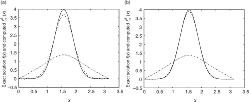
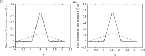
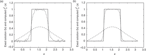
We exhibit the qualitative behaviour of the computed solutions of Examples 2–4 using different noise added into the data (Figures 2–4). Since the direct problem with f given by (36) does not have an analytical solution, the data g is obtained by solving the direct problem using finite difference. Figure 2 shows the numerical solution of the heat source . According to different ϵ, δ given by (32) and the absolute error E(f): (37) are shown in Table 5. From Table 2 we can see even for a relatively high amount of noise added into the data, the numerical results retrieved for the heat source represent good approximations for the exact values. In addition, the numerical heat sources converge towards their corresponding exact solutions as the amount of noise decreases. The scheme works equally well for piecewise smooth and discontinuous heat sources. To illustrate this, the numerical results retrieved for Examples 3 and 4 using different noise added into the data are presented in Figures 3 and 4. From these figures it can be seen that the numerical solution is less accurate than that of Examples 1 and 2. It is not difficult to see that the well-known Gibbs phenomenon and the recovered data near the non-smooth and discontinuities points are not accurate. Note that the same situation happened for the iterative method 9. Taking into consideration the ill-posedness of the problems, the results presented here are quite satisfactory.

Figure 2. Exact solution (solid) and its approximation (dashed) for Example 2. Also, we illustrate the data vector g (dash-dotted). (a) ε = 10^-3; (b) ε = 10^-4.

Figure 3. Exact solution (solid) and its approximation (dashed) for Example 3. Also, we illustrate the data vector g (dash-dotted). (a) ε = 10^-3; (b) ε = 10^-4.

Figure 4. Exact solution (solid) and its approximation (dashed) for Example 4. Also, we illustrate the data vector g (dash-dotted). (a) ε = 10^-3; (b) ε = 10^-4.

Table 5. δ give by (32) and the corresponding error E(f).

ϵ	0.005	0.02	0.03
δ	0.0015	0.0057	0.0091
E(f)	0.2405	0.3729	0.4758

5. Conclusion

The problem of identifying a heat source term in a heat equation is important in many branches of engineering sciences. In this article, we proposed an interesting method which was based on the idea of the quasi-reversibility method. We added a perturbation term in the heat equation with a coefficient that serves as a regularization parameter to stabilize the problem. It is shown that with a certain choice of parameter, an estimate of almost Hölder type is obtained. The numerical results indicate that the proposed method works well for problems with small measurement errors.

Acknowledgements

We are grateful to the reviewers whose constructive comments and criticisms led to improvements of the presentation. The project is supported by the National Natural Science Foundation of China (No.10671085).

References

- Cannon, JR, 1984. One Dimensional Heat Equation. California: Addison-Wesley Publishing Company; 1984.
- Savateev, EG, 1995. On problems of determining the source function in a parabolic equation, J. Inv. Ill-posed Probl. 3 (1995), pp. 83–102.
- Solov'ev, VV, 1990. Solvability of the inverse problem of finding a source, using overdetermination on the upper base for a parabolic equation, Diff. Equ. 25 (1990), pp. 1114–1119.
- Cannon, JR, and Estevz, SP, 1986. An inverse problem for the heat equation, Inverse Probl. 2 (1986), pp. 395–403.
- Li, GS, and Yamamoto, M, 2006. Stability analysis for determining a source term in a 1-D advection-dispersion equation, J. Inv. Ill-posed Probl. 14 (2006), pp. 147–155.
- Yamamoto, M, 1993. Condtional stability in determation of force terms of heat equations in a rectangle, Math. Comput. Model. 18 (1993), pp. 79–88.
- Buryki, AA, and Denisov, AM, 1997. Determination of the unknown sources in the heat-conduction equation, Comput. Math. Model. 8 (1997), pp. 309–313.
- Farcas, A, and Lesnic, D, 2006. The boundary-element method for the determination of a heat source dependent on the variable, J. Eng. Math. 54 (2006), pp. 375–388.
- Johansson, T, and Lesnic, D, 2007. Determination of a spacewise dependent heat source, J. Comput. Appl. Math. 209 (2007), pp. 66–80.
- Ling, L, Yamamoto, M, Hon, YC, and Takeuchi, T, 2006. Indentification of source locations in two-demensional heat equations, Inverse Probl. 22 (2006), pp. 1289–1305.
- Ryaben'kii, VS, Tsynov, SV, and Utyuzhnikov, SV, 2007. Inverse source problem and active shielding for composite domains, Appl. Math. Lett. 20 (2007), pp. 511–515.
- Yi, Z, and Murio, DA, 2004. Source Term identification in 1-D IHCP, Comput. Math. Appl. 47 (2004), pp. 1921–1933.
- Trong, DD, Long, NT, and Alain, PND, 2005. Nonhomogeneous heat equation: Identification and regularization for the inhomogeneous term, J. Math. Anal. Appl. 312 (2005), pp. 93–104.
- Lattès, R, and Lions, JL, 1969. The method of quasi-reversibility: Applications to partial differential equations. New York: Elsevier; 1969.
- Dorroh, JR, and Ru, XP, 1999. The application of the method of quasi-reversibility to the sideways heat equation, J. Math. Anal. Appl. 236 (1999), pp. 503–519.
- Eldén, L, 1987. Approximations for a Cauchy problem for the heat equation, Inverse Probl. 3 (1987), pp. 263–273.
- Xiong, XT, Fu, CL, and Qian, Z, 2006. Two numerical methods for solving a backward heat conduction problem, Appl. Math. Comput. 179 (2006), pp. 370–377.
- Qian, Z, Fu, CL, and Xiong, XT, 2006. Fourth-order modified method for the Cauchy problem for the Laplace equation, J. Comput. Appl. Math. 192 (2006), pp. 205–218.
- Engl, HW, Hanke, M, and Newbauer, A, 1996. Regularization of Inverse Problems. Boston, MA: Kluwer Academic; 1996.
- Kirsch, A, 1999. An Introduction to the Mathematical Theory of Inverse Problems. Berlin: Springer; 1999.
- Landweber, L, 1951. An iteration formula for Fredholm integral equation of the first kind, Am. J. Math. 73 (1951), pp. 615–624.
- Tautenhahn, U, 1998. Optimality for ill-posed problems under general source conditions, Numer. Funct. Anal. Optimiz. 19 (1998), pp. 377–398.
- Qian, Z, 2008. Regularization of inverse problems in mathematical physics, Ph.D. diss.. Lanzhou University; 2008.
- Eldén, L, 1997. Solving an inverse heat conduction problem by ‘Method of lines’, Trans. ASME J. Heat Transfer 119 (1997), pp. 913–923.