Optimal manipulator parameter selection using evolutionary optimization technique

Abstract

This article discusses an approach to selecting the optimal design parameters of a manipulator for minimum performance variations. The variations in desired performance of the manipulator are attributed to the effect of uncertainty in design, process and noise factors. To incorporate the effect of uncertainties in design parameters, a modification in evolutionary optimization approach is proposed. A worst-case approach has been used to model the uncertainties and simulate the performance of the manipulator while performing a task. The design parameters obtained from this optimization process are insensitive to the effect of uncertainties. The proposed approach has been illustrated with the help of a 2-DOF RR planar manipulator. This approach has also been implemented in a genetic algorithm to compare the computational advantage of the proposed modification in the differential evolution technique. The optimal design parameters are observed to be different for different tasks and trajectories in the workspace.

Keywords:

• manipulator performance variations
• control factors
• noise factors
• positional error
• orthogonal array
• evolutionary optimization technique
• differential evolution technique

1. Introduction

There are many industrial applications where a manipulator is required to carry out a precise task with high accuracy. However, industrial manipulators fail to deliver the desired performance because the accuracy of the manipulator is affected by computational error, machining tolerance, joint clearances and misalignment, flexibility effect of links, gear backlash and a host of other static and dynamic effects 1. These effects are called noise factors, which are difficult to model and costly to control 2. Hence, designing an industrial robotic manipulator to satisfy the desired performance requirement is a complex task. In the last decade, the philosophy of developing stable products and processes that exhibit minimum sensitivity to uncontrollable noises has been prevalent in the research community. However, robot manufacturers adopt traditional methods of experimenting with prototypes that are time consuming and expensive to manufacture. To assuage these difficulties an evolutionary optimization approach and mathematical model of the manipulator, i.e. kinematic and dynamic models, are used to obtain the optimal manipulator parameters, which are insensitive to noises. The kinematic and dynamic models of manipulators are non-linear and coupled. Thus, explicit modelling of noises will make the dynamic model still complex. A worst-case approach has been discussed to incorporate the effect of uncertainties and simulate the performance. Subsequently a modification in evolutionary technique has been proposed to incorporate the effect of real world uncertainty and optimize the parameters of the manipulator. The optimized parameter is expected to be insensitive to noises and deliver minimum performance variations.

Many search and optimization techniques are available in literature, but these cannot be used to optimize the robot design parameters i.e. link length, link mass, joint offset and link twist, for optimal performance. The reasons for these difficulties are the non-availability of the objective function, i.e. performance of manipulator, in terms of design parameters, initial guessing solution and information to decide the next point for exploration. To overcome these shortcomings, an evolutionary-based technique is employed. The evolutionary techniques are known for their inability to handle the effect of uncertainty on decision variables, which cause stochastic behaviour. Therefore, to select optimal value and optimize the objective function, a simple modification in the existing evolutionary approach has been proposed. This modification will help in incorporating the effect of uncertainties in decision variables, and in getting a global optimum. The optimal solutions will not vary widely because of stochastic behaviour and number of simulation runs.

1.1. Background of research

There are many pieces of literatures available addressing kinematic error analysis of robot end-effectors, calibration of robot manipulators and parameter optimization of robots for various performance criteria. However, the application of evolutionary techniques to determine optimal parameters of manipulator for minimum performance variations is rare. Khatib and Burdick 3 investigated the dynamic characteristics of manipulators and developed a new method for the optimization of dynamics in manipulator design. Manoochehri and Seireg 4 developed a computer programme for form synthesis and optimal design of a robot manipulator using the dynamic programming approach, while Shiller and Sundar 5 addressed the design of multi degree-of-freedom (DOF) systems for optimal dynamic performance based on the acceleration lines. Khatib and Bowling 6 investigated the problem of manipulator design for increased dynamic performance where dynamic performance of a manipulator is characterized by the inertial and acceleration properties of the end-effector, and used optimization techniques to determine the design parameters which improve manipulator performance. Chocron and Bidaud 7 proposed a method for task-based design of modular robotic systems using genetic algorithms (GA) and introduced a 3D kinematic description for modular serial manipulators and a two-level GA to optimize their topology from task specifications. Stocco et al. 8 proposed a new global isotropy index (GII) to quantify the configuration independent isotropy of a robot's Jacobian or mass matrix and presented a new discrete global optimization algorithm to optimize either the GII or some local measure without placing any conditions on the objective function. Carretero et al. 9 undertook architecture optimization of a three DOF parallel mechanism and demonstrated that specific values of design variables allow minimization of parasitic motion, i.e. motions in the three unspecified motion coordinates. Shiakolas et al. 10 applied three evolutionary techniques to optimize the required torque of robots for a defined motion subject to different constraints. He et al. 11 presented mathematical methods for the placement of serial robot manipulators with respect to pre-defined target points in arc welding applications and proposed an adaptive genetic algorithm (ASAGA) to dynamically modify the parameters of GA in terms of the simulated annealing mechanism. Dolinsky et al. 12 introduced a new inverse static kinematic calibration technique based on genetic programming, which is used to establish and identify model structure and parameters. These research attempts show the applications of evolutionary algorithms (EA) to optimize the kinematic and dynamic parameters. However, the use of EA to optimize the stochastic behaviour of manipulator performance is found to be non-existent.

Applications of EAs, to obtain the optimal decision variables are available in many areas. A few important references dealing with evolutionary-based techniques for product parameter design and optimization have been provided below. Gold and Krishnamurty 13 proposed trade-off-based robust engineering design methodology to experimentally solve a robust optimal solution for a mechanical engineering design problem, using the decision maker's or designer's subjective preferences. Li and Azarm 14 presented an approach wherein product design is viewed as a selection process with two main stages, design alternative generation and design alternative evaluation, and focused on a design alternative evaluation model in that designer's preferences, customers’ preferences and market competition are accounted for, in order to select the best possible design. Hacker and Lewis 15 discussed the optimization of systems with multiple local optima and one or more uncertain design parameters, and presented an approach that utilizes both local and global optimization algorithms to find good design points more efficiently than either could alone. Bagchi 16 used GA to uncover the dependency among the key design factors and obtain robust performance. Ray and Tsai 17 presented a swarm algorithm that is applicable for optimization problems in general, and explored it for airfoil design optimization. The differential evolution (DE) algorithm is a recently developed evolutionary approach proposed by Storn 18–20 for minimizing non-linear and non-differentiable continuous space functions. Later Price and Storn 20 and other researchers presented a generalized algorithm on DE to optimize a variety of problems. This algorithm has been applied to various fields successfully. However, there is no literature on DE that deals with optimization of product performance variations that have stochastic behaviour.

A modification to the existing EA is proposed, which combines the DE optimization technique and orthogonal array (OA) proposed by Taguchi. An OA is a fractional factorial design and is used in design of experiments, which assures a balanced comparison of levels of any factor or interaction of factors 2. In this article, a methodology to select the appropriate OA based on the number of decision variables in the optimization problem is discussed. In addition a method is presented to incorporate the effect of uncertainties in decision variables. This approach uses all evolutionary operators of DE with one modification. The cost function of each population member is evaluated summing the effects of uncertainties created by the selected OA. The proposed approach has been applied to optimize the design parameters of 2-DOF RR planar manipulator for optimum performance. The objective of parameter optimization problem is to minimize the mean positional error considering kinematic and dynamic models of manipulator for a specified task subject to reachability constraints.

This article is organized in five sections. In Section 2, the optimization approach is discussed. The proposed modification in the evolutionary technique for optimal parameter design of manipulator is presented in Section 2.2. In Section 3, the probabilistic approach to simulate the performance of the manipulator is discussed. In Section 4, a proposed approach for optimal parameter design of 2-DOF RR planar manipulator is discussed. Finally, in Section 5, the results of the optimization process are presented and compared with the performance of GA.

2. Optimization approaches

The goal of a product parameter design optimization approach is to find the values of design parameters of the product that deliver the best performance criterion. Due to variations in manufacturing, assembly and other uncertainties, these parameters deviate from their nominal dimension. These variations in parameters lead to variations in performance. The aim of this article is to develop an optimization method, which incorporates the effect of uncertainties in design parameter systematically and achieves the desired objective with less computation. To optimize parameters for reduced performance variations, the DE optimization technique is used. The distinctive features of the proposed technique are the method by which effects of uncertainties are incorporated and cost function is evaluated. This method is discussed below with important features of DE.

2.1. Differential evolution technique

Differential evolution is a search and optimization technique, which works differently, compared to classical search and optimization methods. DE has been increasingly applied to various search and optimization problems in the recent past. Storn 19, proposed the working principle of DE. The advantage of DE is its simple structure, ease of use, speed and robustness.

A cost function, C is used to rate the individual vectors according to their capability to minimize the objective function. DE is a parallel search method that operates on D-dimensional parameter vectors. The number of vectors is equal to user-defined population size. The initial population vector is chosen randomly. The DE process starts by selecting a target vector. Then, it randomly selects two other vectors and generates a difference vector, which is multiplied with a user-defined weighting factor F to obtain the ‘weighted difference vector’. The weighted difference vector and randomly chosen mutation vector are added to create a noisy vector, which is subjected to crossover process with the target vector in order to generate the trial vector. The cost function of the trial vector is then compared with the cost function of the original target vector. The vector having low cost function is allowed into the new population. This process is repeated for all the population members and a new set of population members is created.

From the above explanation, it is evident that the cost function evaluation of members of the population is carried out once and makes it unsuitable for problems which deal with stochastic behaviour. Hence, the following modification is proposed to incorporate the effect of uncertainties and reduce the variability in performance during the optimization process. The desired modification of the DE technique to incorporate the effect of uncertainties of design parameters is discussed below.

2.2. Proposed DE approach

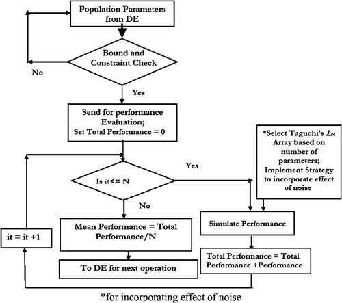
The performance variations of a product are attributed to the effect of noises in design and process parameters. These effects can be modelled by assuming a particular probability distribution function, which the noise factors follow. By this assumption, the amount of computation needed to improve the accuracy of the result of the optimization process would be very high. Therefore, uncertainties ranges (levels) of the design and process parameters (factors) are considered in place of probability distribution of noise parameters. Thus, tolerance associated with the nominal dimensions of each design and process parameter are considered to incorporate the effect of noises. The tolerance of design and process parameters creates a hyper-rectangular design region around the nominal dimensions of design and process parameters. The corner points of the design region are used to simulate performance of the product and these provide a finite set of performance. As opposed to single point designs where every population member results in a particular performance, each candidate design produces a set of performances. To make this possible, systematic use of OA is planned. By use of hyper-rectangular space created by OA, variability in that domain is captured. This evaluation procedure in evolutionary technique provides a ‘worst case’ scenario for the determination of performance variations. Design points (corner point) in the hyper-rectangular region are evaluated for performance and subsequently obtained performances are transformed to provide a cost function. Successively the designs evolve by comparing the cost function for each member of the population. The strategy adopted to handle the effect of noise in the optimization process is shown in Figure 1.

Figure 1. Flow diagram for the proposed evolutionary approach.

The advantage of using OA is that it allows the evolutionary technique to sample only a fraction of the design space, which is efficient as compared to other stochastic optimization methods, such as Monte Carlo simulation. These methods use a large number of sample points to ensure high accuracy.

3. Approach to simulate the performance of manipulator

In manipulator's performance analysis, unknown variations in material distribution, uncertainty in manufacturing and assembly, joint clearances and uncertainty in boundary condition leads to a variation in performance. As it is known that the dynamic model of a manipulator is highly coupled and non-linear, simulation of performance incorporating the effect of noise becomes difficult. Given the randomness of robot parameters, models for their probability distributions are needed. For the sake of conciseness, the variations of the parameter are assumed to obey Gaussian distributions with non-zero mean and non-identical standard deviations. Therefore, the variations in length and mass of the links are assumed to follow the Gaussian distribution and standard deviations are dependent on the specified tolerance for link lengths and link masses.

Robot performing commanded task can be modelled as a stochastic process which is driven by actuators and when the time interval between sample values of supplied torque is small, the process becomes highly correlated over time. As torque supplied to the manipulator joint is in time order and highly correlated, the effect of noise factors on supplied torque by actuators are treated as random vectors. These vectors are assumed to follow Gaussian stochastic process with Markov properties 21. Therefore, supplied torque at manipulator joint is assumed to follow Gaussian stochastic process with Markov properties. Where the future values of a stochastic process depend only on the immediate past or present but not all past events. Thus, a stochastic process with Markov properties is represented mathematically as 22:

The family of random variables {X_tn} indexed by the continuous real variable t and represents points in time, (1) where, X_tn denote the state of the process at time t_n and u_n,u_n − 1,u_n − 2,… are the values of the process parameters. is called transition probability for (u(t)_n + 1 = u_n + 1), given that (u(t₁) = u₁,…,u(t_n) = u_n). The strategy adopted to simulate the joint torque vector is discussed below.

3.1. Simulation of joint torque

As the fluctuation in supplied joint torque vector τ(t) is assumed to follow Gaussian stochastic process with Markov properties, it is simulated as a time series. The time series is a sequence of observations taken sequentially over time. These observations in a time series are regarded as a sample realization from an infinite population of such time series that could have been generated by the stochastic process. The stochastic model, which can be used for simulation of supplied joint torque vector, is the auto-regressive process model. In this model, the current values of the process are expressed as a finite, linear aggregate of previous values of the process and a shock a_t. A generalized autoregressive process 23 of order p is represented as: (2) where the values of the process at equally spaced time t,t − 1,t − 2,… is denoted by τ_t,τ_t − 1,τ_t − 2,… . Also the are the deviation from mean μ; e.g. and the symbol φ₁,φ₂,φ₃,…,φ_p are the finite set of weight parameters. For simulation of random joint torque vector first-order auto-regressive (Markov) process is assumed and Equation (2) becomes (3) where φ₁ is unknown constant and a_t is normally and independently distributed with mean zero and standard deviation σ_a. The observations from such a model have zero mean and standard deviation and the observations that are k periods apart (τ_t and τ_t − k) have correlation coefficient . The relationship between the standard deviation of random shocks σ_ai and the process σ_τi is given by (4) To satisfy the conditions of stationary process, the value of φ₁ is chosen between [ − 1,+ 1], where the stationary process has constant mean and standard deviation over time t.

Therefore, noise parameters used in the simulation process are represented by

i.	Error due to manufacturing and assembly tolerances are specified by standard deviations of Gaussian distribution, i.e. σl1,σl2,σm1 and σm2.
ii.	Fluctuations in supplied joint torque are denoted by standard deviations of Gaussian stochastic process, i.e. στ1 and στ2.
iii.	Viscous friction at the manipulator joints are specified by constants B1 and B2.

The methodology adopted to simulate the performance of the manipulator is discussed next.

3.2. Computation of manipulator performance

The dynamic model of a manipulator is coupled and non-linear therefore, the present approach uses Euler's numerical integration technique to simulate the performance. This approach simulates joint acceleration, velocity and position. The torque vector τ(t) required for the manipulator joints is obtained using inverse dynamics. For the computation of torque vector numerical values of the nominal values of manipulator kinematic and dynamic parameters, Cartesian coordinates of start and destination points, and type of trajectory to reach destination are assumed. Then the actual torque vector available at the individual joints of the manipulator is simulated using method discussed in Section 3.1. The actual output vectors available at joints, i.e. are computed using forward dynamics. These vectors are obtained by integrating the dynamic model numerically. For each time step (sampling time) the effects of noise for each control factor, in the form of individual random error, are generated and incorporated in the respective parameters. The noise parameters like manufacturing and assembly tolerances and fluctuation in supplied torque are incorporated into design and process parameters. Whereas the noise parameters like viscous friction and effect of joint clearances on performance are used individually in integration process. Subsequently joint coordinates q(t) are transformed, using the kinematic models, to obtain the Cartesian coordinates of the point reached at each time step and destination reached. These results are used to compute the positional error at the destination while moving along a trajectory.

4. Optimal design of manipulator parameters

Traditional methods of experimenting with various prototypes are often expensive and are not always successful in complex systems. In order to find optimum manipulator design and process parameters that give minimal performance variations to perform a task, performance deviation at the destination for each experiment ϵ_i is defined.

Positional error: The positional error ϵ_i is defined as: (5) where (x, y, z) and (x_f,y_f,z_f) are the coordinates of the actual and desired point reached by the end-effector during i-th simulation, respectively.

Mean positional error: Mean positional error is defined as: (6) where n is number of experiments or replications and ϵ_i is positional error for i-th experiment. This performance measure provides the information regarding the deviation in performance at the destination while moving along a particular trajectory. Hence, the objective function is expressed mathematically as: (7) The lower and upper values of the link length and mass and reachability of the manipulator are treated as the constraints of the optimization problem. These are specified mathematically as: (8) (9) where l_il,m_il and l_iu,m_iu are the lower and the upper bounds of the length and mass of link i, respectively. The constraints on the joint limits or range of motion of the manipulator are imposed due to physical constraints as: (10) where θ_i is the joint variable for joint i and θ∈Rⁿ is the real valued joint variable with n being the number of joints. It is assumed that the required torque at the joints to perform the specified task is available without any restriction.

4.1. Procedure for robot parameter optimization

The formulation of the optimization problem has already been discussed, where the objective function of the problem, the design parameters and the constraints are identified. For the parameter optimization problem, the desired start and destination point in Cartesian space, time for the motion and type of trajectory and design parameter bound are assumed.

Using the DE algorithm, population members are randomly generated and these values are checked for any constraint violation. If constraints are not violated then design parameters are used to evaluate the objective function (cost function). These evaluations are used in the optimization routine where new values for the design variables are generated. To evaluate the cost function, the strategy discussed in Section 2.2 is used. The effects of noises are incorporated with the help of OA, to generate several design combinations. Each design combination is equivalent to one corner point of the hyper-rectangular region created by OA.

These designs’ points are utilized to simulate the performance, i.e. positional error at the target point. To simulate performance at the destination, the steps discussed in Section 3.2 are followed. By this process, the performance of one design combination, i.e. one corner point of hyper-rectangular space, is evaluated. After computing the performance at all the corner points of this space, the mean positional error is computed. Then the mean positional error obtained becomes the cost function for one population member. Subsequently all population members are evaluated to get cost function. In addition, these cost functions provide value for comparison of design variables in the optimization process. This process is repeated until the criterion for the number of generations is met.

4.2. Parameter design optimization of 2-DOF RR planar manipulator

The proposed approach is illustrated by selecting optimal parameters of 2-DOF RR planar manipulator. The optimization problem for the 2-DOF RR planar manipulator has been formulated as given in Equations (7–10). As the manipulator works in the xy plane the positional error ϵ_i becomes (11)

For mean positional error, Equation (6) is used, subject to the constraints discussed in Equations (8) and (9).

Check for reachability of manipulator: In addition to the constraints discussed while searching for the optimal design, it must be ensured that the task to be performed lies within the range of workspace. Thus, it should satisfy the conditions given below: (12) (13) where . If the Cartesian coordinates for a manipulator satisfy the above conditions, then it is considered reachable and the design parameter vector generated by DE participates in the optimization process.

4.2.1. Kinematic and dynamic models of 2-DOF RR planar manipulator

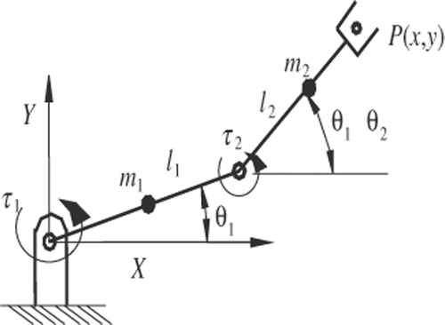
Conducting experiments to determine optimal parameters are very costly and uneconomical. Along with this difficulty, the measurements of performances are costlier still and difficult to measure. For an illustration of the approach, 2-DOF RR planar manipulator shown in Figure 2 is considered.

Figure 2. A 2-DOF RR planar manipulator and its parameters.

The kinematic model in terms of D–H (Denavit–Hartenberg) notation for the homogenous transformation matrix 24 is given by: (14) where with i, j = 1, 2 for the two links, link 1 and link 2, respectively, and l₁ and l₂ are lengths of two links. The coordinates of end-effector position P(x,y) are obtained from last column of (14). The links are assumed rigid thin rods with gravity loading. Based on Lagrange–Euler formulation the dynamic behaviour of joint i of the manipulator with contributions of viscous friction is given by 24: (15) where M_ij the symmetric inertia matrix, h_ijk the centrifugal and coriolis force coefficients, G_i the gravity force vector, τ(t) the joint torque vector and are the joint position, velocity, acceleration vectors, respectively. Therefore, torque equations for the two joints in generalized form are: (16) (17) where where are angular displacements, velocities, accelerations of link 1 and 2, respectively; m₁ and m₂ are masses of link 1 and link 2, respectively, and g is the acceleration due to gravity.

Based on the trajectory chosen to perform the task, the torque required at joints are determined. The two trajectories used for the exploration are discussed below.

Trajectory I–cubic path: For the manipulator to follow a cubic trajectory, the initial (i) and final (f) boundary conditions are: q_i = (θ_1i;θ_2i); q_f = (θ_1f;θ_2f); where q_i,q_f are joint coordinates and are joint velocities, respectively, and time to reach the destination is T_g. The time law of cubic trajectory is given 24 by: (18) where a₀,a₁,a₂,a₃,b₀,b₁,b₂,b₃ are constants. Applying boundary conditions to (18), the constants are computed.

Trajectory II–quintic path: For the manipulator to follow a quintic trajectory, the boundary conditions are: where are joint accelerations, respectively. The time law of quintic trajectory is given 25 by: (19) where a₀,a₁,a₂,a₃,a₄,a₅,b₀,b₁,b₂,b₃,b₄,b₅ are constants. Applying boundary conditions to (19), the constants are computed. Using (18) for cubic time law and (19) for quintic time law in dynamic model of manipulator, τ(t) is computed.

The closed form solutions are difficult to obtain, the torque obtained from inverse dynamics are integrated to compute the joint coordinates, velocities and accelerations with the effect of noise. In this work the Euler numerical integration method 25 has been applied for obtaining angular velocities and angular positions from angular accelerations.

5. Simulation and discussion

The evolutionary optimization approach is implemented in MATLAB. The numerical values for different parameters are assumed and given below. To determine the influence of task specifications on optimal parameter design, a number of cases has been considered. The task specification for deterministic cases and cases with the effect of noise are provided in Tables 1 and 2, respectively.

Table 1. Manipulator task specifications for the deterministic case.

Trajectory	Coordinates of start point (xim,yim)	Coordinates of destination point (xfm,yfm)	Time to travel (s)
Cubic	(0.65, 0)	(0.4, 0.3)	2
Quintic	(0.65, 0)	(0.4, 0.3)	2

5.1. Assumed process parameters

For the simulation of the performance of a manipulator, different tasks as given above are assumed.

i.	Weight parameter for first-order auto-regressive process φ1 = 0.8.
ii.	Time step for numerical integration = 0.001 s.
iii.	Values of viscous friction at joints, B1 and B2 are 2 and 3.5 Ns/m, respectively.

The constraints imposed during optimization process for the deterministic case and cases with the effect of noise, are given in Table 3. These constraints are assumed to be the same for all tasks.

Figure 3. Function history of deterministic case for cubic trajectory.

Figure 4. Function history of deterministic case for quintic trajectory.

Table 2. Manipulator task specifications for case with effect of noise.

Case	Coordinates of start point (xim,yim)	Coordinates of destination point (xfm,yfm)	Time to travel (s)
(i)	(0.65, 0)	(0.4, 0.3)	2
(ii)	(0.65, 0.05)	(0.4, 0.3)	2
(iii)	(0.65, 0.1)	(0.4, 0.3)	2
(iv)	(0.65, 0.05)	(−0.4, 0.3)	2
(v)	(0.65, 0.1)	(−0.4, 0.3)	2
(vi)	(0.4, 0.3)	(0.65, 0)	2

Table 3. Parameter constraints for manipulator.

Link 1 length l1 range (m)	Link 2 length l2 range (m)	Link 1 mass m1 range (kg)	Link 2 mass m2 range (kg)

The optimization of the deterministic case, while following cubic and quintic trajectories are carried out using the method discussed in Section 2.1. The evolution control parameters used for optimization are selected with the help of the trial and error method. In addition, rules to select control parameters specified by Storn 19 are followed. Selected control parameters for DE are population size (NP) = 40, no. of generations (N) = 50, crossover probability (CR) = 0.5, weighting factor (F) = 0.8.

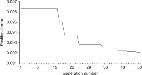
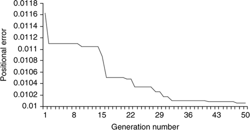
In deterministic optimization, the evaluation of cost function for each population member is carried out once because during simulation of performance, the effect of noise is not considered. In this process the positional error obtained from simulation is computational error. Hence, by application of the DE technique the design parameter, which minimizes computational error, is obtained. The generation-wise reduction in positional error, i.e. computational error is provided in Figures 3 and 4, respectively. In Figure 3, it is observed that the positional error reduces from 0.0965 × 10^− 2 m to 0.0921 × 10^− 2 m for the specified task following cubic trajectory. Similarly, from Figure 4 it is observed that the positional error reduces from 0.0116 × 10^− 2 m to 0.0101 × 10^− 2 m for the task following quintic trajectory. Cubic trajectory is jerky compared to quintic trajectory. Thus, the positional error for the cubic trajectory is more than the positional error for quintic trajectory. The optimal parameter values for deterministic cases are specified in Table 4.

Table 4. Optimal parameters of manipulator for the deterministic case.

Trajectory	Link 1 length l1 (m)	Link 2 length l2 (m)	Link 1 mass m1 (kg)	Link 2 mass m2 (kg)	Function value × 10^− 2(m)
Cubic	0.4502313	0.44993491	6.255106	7.985928	0.092029
Quintic	0.54994198	0.41548853	9.975794	4.014191	0.010061

It can be seen that the optimal parameter value obtained using the DE technique provides a different solution for different trajectories. Subsequently, to obtain the optimal design parameters which deliver optimized real life performance, the proposed approach is applied. For these cases, the effect of noise is incorporated while simulating the performance, subsequently taken into consideration in the optimization process. The tasks considered for this optimization process are provided in Table 2. The evolution control parameters for this case are chosen to be same as deterministic optimization. Another important aspect of the population-based optimization method is average history of performance, where an algorithm is run with different initial populations a specified number of times to observe the average histories over the multiple runs. Interestingly the solution is observed to be very close to what was achieved on other occasions. Therefore, it was decided to run the above algorithm once to illustrate the use.

There are six control factors (lengths of the two links, its corresponding masses and fluctuations in joint torques). Correspondingly, for these control factors there will be six noise parameters. Since there are six noise parameters and two levels for each parameter (−3 sigma and +3 sigma), 2⁶ combinations are possible and conducting all experiments is impractical and leads to increased computation time. To reduce the amount of computation and incorporate the effect of noise systematically, Taguchi's OA 2 is selected. The rationale behind this selection is the number of factors for which the effect of noise needs to be incorporated. In the present article, only the effect of link length and link mass variation is incorporated in the optimization process. For the assumed tolerances of each design parameter and specific parameter values of each parameter, the OA selected provides noise to each parameter. The noises are deviations of the tolerance value from nominal parameter value. These represent ‘worst case’ tolerance deviations and satisfy the 3-sigma limits of normal Monte Carlo variability. Each row of OA is a noise combination that is treated as repetitive data for each member of population. To incorporate the effect of noise 1's and 2's of L₈ array presented in Table 5 have been used. These numbers provide the direction in which the population parameter vector deviates from the specified values. The assumed noises of six parameters are specified in Table 6. These noises are utilized in DE to incorporate noise in simulation and optimization process. The detailed use of OA in DE has been provided in Tables 7–9. To explain the use of OA in DE approach, an example has been considered. In which all the eight possible combinations are generated for the set of four parameters l₁, l₂, m₁ and m₂. The assumed tolerances for link lengths l₁, l₂ and masses m₁, m₂ are provided in Table 7 and the assumed parameter vector values sent by DE for optimization are specified in Table 8. The resulting eight combinations with the use of L₈ array are given in Table 9.

Table 5. L₈ Orthogonal array.

Experiment no.	Column number
1	2	3	4	5	6	7
1	1	1	1	1	1	1	1
2	1	1	1	2	2	2	2
3	1	2	2	1	1	2	2
4	1	2	2	2	2	1	1
5	2	1	2	1	2	1	2
6	2	1	2	2	1	2	1
7	2	2	1	1	2	2	1
8	2	2	1	2	1	1	2

Table 6. Noise for design and process parameters.

Parameters	Tolerances
Lengths of link l1 and l2 (m)	±0.0003
Mass of link m1 and m2 (kg)	±0.015
Torque at joint τ1 and τ2 (Nm)	±0.05

Table 7. Assumed tolerances for control factors.

Parameters	Tolerances
Link lengths l1, l2 (m)	±0.0003
Link masses m1, m2 (kg)	±0.015

Table 8. Assumed population member values sent by DE.

l1 (m)	l2 (m)	m1 (kg)	m2 (kg)
0.425	0.375	6	4

Table 9. Combinations created from the population member values using OA.

Experiment no.	Parameters
l1 (m)	l2 (m)	m1 (kg)	m2 (kg)
1	0.4247	0.3747	5.985	3.985
2	0.4247	0.3747	5.985	4.015
3	0.4247	0.3753	6.015	3.985
4	0.4247	0.3753	6.015	4.015
5	0.4253	0.3747	6.015	4.985
6	0.4253	0.3747	6.015	4.015
7	0.4253	0.3753	5.985	3.985
8	0.4253	0.3753	5.985	4.015

The experiment is conducted for each combination and the average of all the experiments is taken. This outcome, i.e. mean positional error, from experiments is sent for comparison in DE optimization process. It is important to mention that the noise in supplied torque is modelled as Gaussian stochastic process with Markov property. Thus to incorporate the effect of noise, assumed standard deviation (tolerance) of fluctuation in supplied torque is used in the simulation. These parameters are not assigned to columns of L₈ OA. The results of the optimization process utilizing the evolutionary technique are presented in Tables 10 and 11.

Table 10. Optimal parameters for cubic trajectory with DE.

Case	Link 1 length l1 (m)	Link 2 length l2 (m)	Link 1 mass m1 (kg)	Link 2 mass m2 (kg)	Mean positional error × 10^− 2 (m)	Number of function evaluations	Time for 50 generations (s)
(i)	0.45115423	0.44025207	6.585616	7.886889	0.130762	698	146580
(ii)	0.4516324	0.44804167	7.843923	7.99053	0.120789	796	167160
(iii)	0.45044698	0.35094645	6.191169	7.998867	0.231646	812	170520
(iv)	0.45021022	0.35036626	6.257418	7.95036	0.236336	728	152880
(v)	0.45713918	0.44867156	6.727582	7.969148	0.111177	764	160440
(vi)	0.45083597	0.44943789	6.037671	7.714803	0.125251	735	154350

Table 11. Optimal parameters for quintic trajectory with DE.

Case	Link 1 length l1 (m)	Link 2 length l2 (m)	Link 1 mass m1 (kg)	Link 2 mass m2 (kg)	Mean positional error × 10^− 2 (m)	Number of function evaluations	Time for 50 generations (s)
(i)	0.53526522	0.44429454	9.728534	7.9974	0.120093	694	145740
(ii)	0.53052684	0.44841063	9.185676	7.976033	0.101264	812	170520
(iii)	0.52195604	0.44669770	9.498453	7.947742	0.097292	812	170520
(iv)	0.45139675	0.44965546	9.898766	7.609616	0.252178	726	152460
(v)	0.45054925	0.44976276	9.920583	7.85658	0.218845	754	158340
(vi)	0.45159362	0.44882879	9.955927	7.763131	0.054702	755	158550

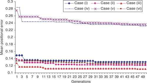
In these tables, the optimal values of the design parameters, the functional value, number of function evaluations and CPU time for 50 generations are presented. This algorithm has been implemented on a computing machine with 1.8 Ghz, 256 MB and RAM capacity. It is observed that the DE approach consistently obtains a smaller function value with less function evaluations. The number of function evaluations is an indication of the computing effort required to reach the optimum function value for the same number of generations. The objective function history for tasks following cubic trajectory are shown in Figure 5.

Figure 5. Function history for cubic trajectory with DE.

In all these cases, the objective function value reduces monotonically. For case (i) following cubic trajectory the cost function, i.e. mean positional error reduces from 0.149 × 10^− 2 m to 0.131 × 10^− 2 m in 50 generations. Similarly for case (ii) the mean positional error reduces from 0.14 × 10^− 2 m to 0.12 × 10^− 2 m. For case (iii) cost function reduces from 0.128 × 10^− 2 m to 0.112 × 10^− 2 m. The objective function value is observed to reduce from 0.284 × 10^− 2 m to 0.236 × 10^− 2 m and 0.273 × 10^− 2 m to 0.238 × 10^− 2 m for cases (iv) and (v), respectively.

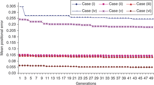
The objective function history for all tasks following quintic trajectories are shown in Figure 6. It is observed that the cost function converges in a monotonic fashion. For the case (i) cost function is observed to reduce from 0.101 × 10^− 2 m to 0.125 × 10^− 2 m. Similarly, for cases (ii) and (iii) the mean positional error is found to reduce from 0.1015 × 10^− 2 m to 0.0972 × 10^− 2 m and 0.1052 × 10^− 2 m to 0.1015 × 10^− 2m, respectively. For cases (iv) and (v) the manipulator performance is found to reduce from 0.305 × 10^− 2 m to 0.255 × 10^− 2 m and 0.250 × 10^− 2 m to 0.220 × 10^− 2m, respectively. The mean positional error is observed to reduce from 0.061 × 10^− 2 m to 0.055 × 10^− 2 m for case (vi). Referring to these, Figures 5 and 6, assumed tasks can be classified into two sections. The tasks (iv) and (v) and the tasks (i)–(iii) and (iv) are observed to deliver a similar type of behaviour.

Figure 6. Function history for quintic trajectory with DE.

5.2. Optimal parameters of manipulator using GA

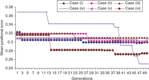
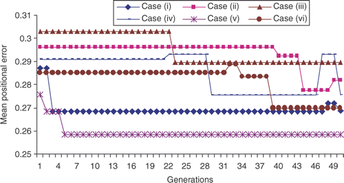
To compare the performance of the above approach, the same modification is implemented in GA. In this case, evaluation of the fitness function is done in the discussed manner. The rest of the steps remain same as discussed in Deb 26. The control parameters are selected based on a trial and error method for which this method provides an optimal solution with less computation and time. The control parameter values are chosen as: NP = 40, cross over probability = 0.8 and mutation probability = 0.175. Using same parameter bounds, noises, tasks and numerical values, a computer program is developed and simulations are run. To compare the performance of GA, a simulation is run for 50 generations. The results of this optimization process are presented in Tables 12 and 13 for the manipulator performing tasks using cubic/quintic trajectory. Similarly, a function history of GA is presented in Figures 7 and 8.

Figure 7. Function history for cubic trajectory with GA.

Table 12. Optimal parameters for cubic trajectory from GA.

Case	Link 1 length l1 (m)	Link 2 length l2 (m)	Link 1 mass m1 (kg)	Link 2 mass m2 (kg)	Mean positional error × 10^− 2 (m)	Number of function Evaluations	Time for 50 generations (s)
(i)	0.50090856	0.44894164	7.706868	7.627576	0.298985	3030	636300
(ii)	0.47413563	0.44741994	9.953008	7.720614	0.299325	3030	636300
(iii)	0.54346479	0.43160096	6.322149	7.602735	0.309823	3030	636300
(iv)	0.45234867	0.36078641	7.03435	7.697754	0.249708	3030	636300
(v)	0.53186493	0.43093319	9.415876	7.70108	0.303738	3030	636300
(vi)	0.52985308	0.42991547	7.672331	4.650942	0.273784	3030	636300

Table 13. Optimal parameters for quintic trajectory from GA.

Case	Link 1 length l1 (m)	Link 2 length l2 (m)	Link 1 mass m1 (kg)	Link 2 mass m2 (kg)	Mean positional error × 10^− 2 (m)	Number of function evaluations	Time for 50 generations (s)
(i)	0.53524039	0.42170688	7.675625	7.908822	0.268773	3030	636300
(ii)	0.50382344	0.41220353	7.517503	4.441751	0.277632	3030	636300
(iii)	0.54346479	0.43160096	6.322149	7.602735	0.289652	3030	636300
(iv)	0.53005154	0.42992842	6.672026	6.639223	0.27548	3030	636300
(v)	0.52977983	0.35500796	7.660979	4.705873	0.258589	3030	636300
(vi)	0.51232633	0.38042798	7.277755	5.522419	0.269944	3030	636300

In all these cases, the objective function value reduces monotonically. After 50 generations, the mean positional error value ranges from 0.3236 × 10^− 2 m to 0.2525 × 10^− 2 m for the tasks, which follow a cubic trajectory. Similarly, the mean positional error ranges from 0.282 × 10^− 2 m to 0.2654 × 10^− 2 m for the tasks, which follow a quintic trajectory.

Figure 8. Function history for quintic trajectory with GA.

Finally from Figures 5 and 6, a monotonic decrease in objective function value is observed. Likewise, in Figures 7 and 8, the objective function value decreases with a slight fluctuation at the start or at the end. But these results are obtained after 3030 number of functional (NOF) evaluations. In the case of DE the NOFs required to reach optimal solution are less. These lead to a reduction in computation time. This is one of the important outcomes of the investigation.

It is observed that the optimal design parameters are different for different tasks. The manipulator is required to perform several tasks; therefore, design of a manipulator to deliver optimal performance in all types of task will be difficult. One of the possibilities is to design the manipulator for a worst-case situation. In all the cases, the cost function is observed to reduce in a monotonic fashion. This behaviour ensures that the DE algorithm with proposed modification can obtain the optimal parameter value with less NOFs and can be used for product shape optimization.

6. Conclusion

An evolutionary optimization approach has been proposed which couples DE optimization techniques with OA of the Taguchi method to incorporate real world uncertainties into optimal parameter design. The design optimization process uses the kinematic and dynamic models of the manipulator. The objective is to minimize the mean positional error of the manipulator, subject to constraints on link design parameters (length and mass). In this article, the DE optimization approach has been applied to obtain optimal parameter design of 2-DOF RR planar manipulator. The results of the above approach are presented and compared with the performance of GA. The results indicate that the DE converges quickly with a lower number of generations and function evaluations. This approach is suitable for optimal manipulator parameter design with the effect of noises. The fast performance of DE indicates that this approach can be a viable optimization technique for processes where development of the objective function is difficult.

References

- Spong, MW, and Vidyasagar, M, 1989. Robot Dynamics and Control. Singapore: John Wiley & Sons; 1989.
- Park, SH, 1998. Robust Design and Analysis for Quality Engineering. London: Chapman and Hall; 1998.
- Khatib, O, and Burdick, J, 1987. Optimization of dynamics in manipulator design: The operational space formulation, Int. J. Robot. Autom. 2 (1987), pp. 90–98.
- Manoochehri, S, and Seireg, AA, 1990. A computer based methodology for the form synthesis and optimal design of robot manipulators, ASME J. Mech. Design 112 (1990), pp. 501–507.
- Shiller, Z, and Sundar, S, 1993. Design of multi-degree-of-freedom mechanisms for optimal dynamic performance, ASME J. Mech. Design 115 (1993), pp. 199–206.
- Khatib, O, and Bowling, A, 1996. Optimization of the inertial and acceleration characteristics of manipulators. MN, USA: Proceedings of IEEE International Conference on Robotics and Automation; 1996, Vol. 4, pp. 2883–2889.
- Chocron, O, and Bidaud, P, 1997. Genetic design of 3D modular manipulators. Albuquerque, NM, USA: Proceedings of IEEE International Conference on Robotics and Automation; 1997, Vol. 1, pp. 223–228.
- Stocco, L, Salcudean, SE, and Sassani, F, 1998. Fast constrained global minimax optimization of robot parameters, Robotica 16 (1998), pp. 595–605.
- Carretero, JA, Podhorodeski, RP, Nahon, MA, and Gosselin, CM, 2000. Kinematic analysis and optimization of a new three degree-of-freedom spatial parallel manipulator, J. Mech. Design 122 (2000), pp. 17–24.
- Shiakolas, PS, Koladiya, D, and Kebrle, J, 2002. Optimum robot design based on task specifications using evolutionary techniques kinematic, dynamic, and structural constraints, Inverse Probl. Eng. 10 (2002), pp. 359–375.
- He, G, Gao, H, Zhang, G, and Wu, L, 2006. "Using adaptive genetic algorithm to the placement of serial robot manipulator". In: Proceedings of the IEEE International Conference Engineering Intelligent Systems. IEEE; 2006. pp. 1–6, DOI 10.1109/ICEIS.2006.1703222.
- Dolinsky, JU, Jenkinson, ID, and Colquhoun, GJ, 2007. Application of genetic programming to the calibration of industrial robots, Comput. Ind. 58 (2007), pp. 255–264.
- Gold, S, and Krishnamurty, S, Trade-offs in robust engineering design. Presented at Proceedings of DETC’97, ASME Design Engineering Technical Conferences. Sacramento, California, September 14–17, 1997.
- Li, H, and Azarm, S, 2000. Product design selection under uncertainty and with competitive advantage, J. Mech. Design 122 (2000), pp. 411–418.
- Hacker, K, and Lewis, K, Robust design through the use of a hybrid genetic algorithm. Presented at Proceedings of DETC’02, ASME Design Engineering Technical Conferences and Computers and Information in Engineering Conference. Montreal, Canada, September 29–October 2, 2002.
- Bagchi, TP, 2003. Multiobjective robust design by genetic algorithms, Mater. Manuf. Process. 18 (2003), pp. 341–354.
- Ray, T, and Tsai, HM, 2004. Swarm algorithm for single- and multiobjective airfoil design optimization, AIAA J. 42 (2004), pp. 366–373.
- Storn, R, 1995. Differential evolution–a simple and efficient heuristic for global optimization over continuous spaces, J. Global Optim. 11 (1995), pp. 341–359.
- Storn, R, 1995. Differential Evolution Design of an IIR-filter with Requirements for Magnitude and Group Delay. Berkeley, CA: International Computer Science Institute; 1995.
- Price, K, and Storn, R, 1997. A simple evolution strategy for fast optimization, Dr Dobb's J. 264 (1997), pp. 18–24.
- Rao, SS, and Bhatti, PK, 2001. Probabilistic approach to manipulator kinematics and dynamics, Reliab. Eng. Syst. Safe. 72 (2001), pp. 47–58.
- Hoel, PG, Port, SC, and Stone, CJ, 1986. Introduction to Stochastic Processes. Boston, USA: Houghton Mifflin Company; 1986.
- Box, GEP, Jenkins, GM, and Gregory, CR, 1994. Time Series Analysis: Forecasting and Control. Singapore: Pearson Education Inc.; 1994.
- Mittal, RK, and Nagrath, IJ, 2003. Robotics and Control. New Delhi: Tata McGraw-Hill Publishing Company Limited; 2003.
- Craig, JJ, 1989. Introduction to Robotics Mechanics and Control. Singapore: Pearson Education Inc; 1989.
- Deb, K, 2003. Optimization for Engineering Design: Algorithms and Examples. New Delhi: Prentice Hall of India Private Limited; 2003.