Abstract
In this study, three different versions of the finite element method (FEM) based on Trefftz functions are presented for solving transient two-dimensional inverse heat conduction problems. The following cases are considered: (a) FEM with the condition of continuity of temperature in the common nodes of elements, (b) no temperature continuity at any point between elements and (c) nodeless FEM. Instead, in each finite element the temperature is approximated by a linear combination of Trefftz functions. These investigations are carried out using temperature data obtained from numerical simulations, exact and disturbed. For the inaccurate data some efficient method of smoothing is presented.
1. Introduction
In most of the papers where the finite element method (FEM) is used to numerically solve problems of unknown temperature field, the boundary conditions are known Citation1–3. The case of a steady heat conduction problem is easier to consider. In the case of transient problems, the use of FEM usually results in extremely large and sparse linear systems of equations Citation4.
The inverse heat conduction problem (IHCP) consists in the estimation of the surface temperature and/or heat flux history, given one or more interior measured temperatures. The IHCP is much more difficult to solve than the direct heat conduction problem in which the initial and boundary conditions are given and the temperatures are to be determined.
There have been various approaches to the IHCP. They are reported widely in Citation5. Some of the approaches were the following: the use of Laplace transform Citation6, the use of Helmholtz equation Citation7, the finite difference method Citation8, the finite element approaches Citation9,Citation10, Tikhonov regularization method Citation11 and Alifanov iterative regularization Citation12.
From the point of view of the inverse problems, an approach based on Trefftz functions (T-functions) seems to be crucial Citation13–15. The T-functions satisfy the governing equations modelling the problem under consideration; therefore, they are better for choosing the so-called shape functions than others. The characteristic feature of the earliest application of the Trefftz method in the FEM context was that the use of the T-functions was confined to a particular part of the domain, Citation16,Citation17. For the problems of heat conduction a relatively complete comparison of different time-progression schemes was performed in Citation18.
One of the first uses of the T-functions to solve the inverse problems of heat conduction was presented in two doctor's dissertations, Citation19,Citation20. Application of the T-functions as basic function of FEM to solving the IHCP was reported in Citation21,Citation22. Then, in Citation23, the FEM with Trefftz (FEMT) functions was combined with an energetic approach. Moreover, the FEMT was compared with the classic FEM. As one could expect, in the case of the inverse problem with unknown temperature on the part of the boundary the classic FEM is useless. On the contrary, the use of the FEMT gave very good results even in the case of inaccurate input data (temperature internal response).
New advanced computational methods based on the meshless approximations have been applied to IHCPs in Citation24.
In this study, three different versions of the FEMT are presented in solving transient two-dimensional IHCPs. The following cases are considered: (a) FEMT with the condition of continuity of temperature in the common nodes of elements, (b) no temperature continuity at any point between elements and (c) nodeless FEMT. Exact, as well as inaccurate input data are considered. Three kinds of physical aspects that regularize the solution are used in the work, Citation25. The first is the minimization of heat flux jump between the elements, the second is the minimization of the defect of energy dissipation on the border between elements and the third is the minimization of the intensity of numerical entropy production between elements. Moreover, smoothing of the inaccurate temperature internal response with the use of T-functions appears to be a very efficient method ensuring stable solution of the considered IHCP. The results show efficiency of both the FEMT (especially in the case of the nodeless approach) and the smoothing with the use of T-functions.
2. The considered problem
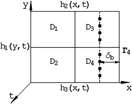
We consider a transient 2D IHCP in dimensionless coordinates in the unit square. On two sides of the square the heat flux is prescribed, whilst temperature is prescribed on a third side. Thermal conditions on the fourth side are unknown. Instead, inside the square on a line distant at δb ∈ (0,0.99) from the side with unknown temperature the internal temperature responses (ITRs) are prescribed.
In the case of transient problem the heat conduction equation is considered
(1)
with the conditions
(2)
(3)
(4)
(5)
(6)
Here Tik's stand for known ITRs in points distant at δb ∈ (0,0.99) from the side x = 1 of the square, i = 1, …, I; k = 1, …, K.
We can consider norms of inaccuracies of the approximate temperature field and the identified boundary temperature, because the exact solution is known.
3. Variants of FEM
In all variants of FEM considered here, the domain is divided into subdomains in which we take linear combination of T-functions as an approximation of the solution. The T-functions, also called solving functions, for transient problems have been introduced in Citation19,Citation20; different T-functions and their applications in mechanics of solids are widely described in monograph Citation21 and in many other papers (compare, e.g. Citation26–28).
In the transient heat conduction problems considered in Cartesian coordinates, the T-functions are called heat polynomials. For 2D problems they are defined as follows:
(7)
where
(8)
and
.
For stationary problems, equation (1) becomes the Laplace equation and the harmonic functions are given in Citation21.
The FEM needs to be given base functions. It is quite obvious that the T-functions are a good choice for base functions because they fulfill the governing equation.
The following cases of FEM are considered:
1. FEMT with the condition of continuity of temperature in the common nodes of elements (): We consider time-space finite elements. The approximate temperature in an j-th element is a linear combination of the T-functions:
| |||||
2. No temperature continuity at any point between elements (): In this case, in order to ensure the physical sense of the solution, we minimize the inaccuracy of the temperature on the borders between elements. | |||||
3. Nodeless FEMT: The time interval is divided into subintervals. In each subinterval the domain Ω is divided into J subdomains (finite elements) and in each subdomain Ωj, j = 1, 2, …, J, the temperature is approximated by the linear combination of the T-functions according to formula (9). The dimensionless time belongs to the considered subinterval. In the case of the first subinterval an initial condition is known. For the next subintervals the initial condition is understood as the temperature field in the subdomain Ωj at the final moment of time in the previous subinterval. The mean-square method is used to minimize the inaccuracy of the approximate solution on the boundary, in the initial moment of time and on the borders between elements. This way the unknown coefficients of the combination, | |||||
Figure 1. Time-space elements in the case of temperature continuous in the nodes.
Moreover, energetic minimization is used to improve the approximate solution, i.e. on the border between elements the defect of energy dissipation, the numerical entropy production or the heat flux jumps are minimized.
Figure 2. Time-space elements in the case of temperature discontinuous in the nodes.
4. The mean-square method and energetic minimization
The time-space elements are presented in . To ensure physical meaning of the approximate solution the energetic minimization is used. Three kinds of minimizing terms are considered:
| • | minimizing the heat flux inaccuracy between elements:
| ||||
| • | minimizing numerical entropy production between elements:
| ||||
| • | minimizing the defect of energy of dissipation between elements:
| ||||
The functional describing mean-square fitting of the approximated temperature field to the initial and boundary conditions (including the temperature jump on the borders between elements) together with one of the three aforementioned minimizing terms has the following form:
(11)
Here JHF denotes the functional describing the heat flux inaccuracy between elements:
(12)
JEP is the functional describing numerical entropy production on the borders between elements
(13)
and JDE stands for the functional describing energy of dissipation between elements
(14)
In order to find the unknown coefficients , the functional J with one of the additional terms depending on the inaccuracy of entropy production, energy dissipation or heat flux on the borders between elements is minimized.
In the case when the functional JHF is taken as the additional term in the functional J, the necessary condition of the functional minimum leads to a system of linear algebraic equations which are not difficult to solve. If the system of equations is ill-conditioned, the solution can be found using the Tikhonov regularization Citation11.
The situation is more complicated when one of the two other functionals is taken as the additional term. Because the integrands in these two functionals are nonlinear functions, the integrals are then replaced with sums according to the Riemann summation. The system of algebraic equations obtained as a result of comparing the partial derivatives of the functional J to zero is then a nonlinear one. Such a system is solved using the Newton method. As a starting point for the Newton method, a solution for the functional JHF is taken.
5. Error of approximation
In order to check the accuracy of three cases of FEM with the minimizing terms, the transient test problem is considered. Because the exact solution is known, the error of the approximate solution in the square in the time-space domain Ω = {(x, y, t) ∈ R3 : 0 ≤ x ≤ 1; 0 ≤ y ≤ 1; 0 < t < te} can be described using the following norms:
(15)
(16)
(17)
The error on the part of the boundary where the temperature is calculated according to the norm reads
(18)
6. Analysis of the problem
6.1. Exact values of the ITRs
At first we consider the problem (1–6) with the exact values of ITRs. The exact solution of the problem reads
The dimensionless time interval is (0,0.01]. The temperatures are known for t ∈ {0.0025, 0.0050, 0.0075, 0.01} at points (1 − δb, yi) with yi ∈ {0.1, 0.2, 0.3, 0.4, 0.6, 0.7, 0.8, 0.9} and δb ∈ (0,0.99). For δb = 0 the problem becomes a direct (initial-boundary) one.
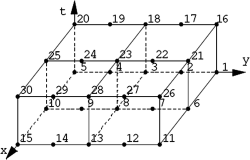
The square has been divided into four elements (). It means that we are looking for an approximate solution in the first four time-space elements (for the first time step) with 12 nodes (compare and ). The time co-ordinates of the nodes are 0 and 0.01, i.e. the time step Δt = 0.01.
Figure 3. The boundary conditions (3–5), the ITR placement and the finite elements.
In the case of nodeless FEMT, the formula (9) with 12 T-functions has been used to describe approximately the temperature field in the element.
The boundary temperature at x = 1 and the temperature field in the square have been calculated with the use of the three aforementioned methods. The errors of the methods according to the temperature field in the square are presented in Tables for FEMT with the condition of continuity of temperature in the common nodes of elements, for FEM with no continuity of temperature in nodal points and for nodeless approach, respectively.
Table 1. Norms of errors of the approximated temperature field as a function of the distance δb from the boundary x = 1 for different energetic minimizing terms and for FEM with the condition of continuity of temperature in the common nodes.
Table 2. Norms of errors of the approximated temperature field as a function of the distance δb from the boundary x = 1 for different energetic minimizing terms and for FEM with no continuity of temperature in the common nodes.
Table 3. Norms of errors of the approximated temperature field as a function of the distance δb from the boundary x = 1 for different energetic minimizing terms and for nodeless FEM.
Comparing the results presented in the Tables one can see that the smallest errors of the temperature field in the square in all three norms are obtained for the nodeless FEMT. The results slightly depend on the regularizing term, but the heat flux jumps minimization seems to be most efficient one.
Sometimes results obtained for δb = 0 (a direct problem) are worse than those for δb > 0 (an inverse problem). It may be a result of approximating the solution with a small number of T-functions; sometimes, in such case, the results inside the region under consideration are better than those close to the boundary.
Errors of the identified temperature at the boundary x = 1 for δb = 0 (0.1) 0.9 and for δb = 0.99 are shown in . The results are almost independent on the FEMT and on the energetic minimizing term.
Table 4. Errors of the identified temperature at the boundary x = 1 for δb ∈ (0, 0.99).
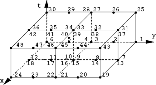
Now let us consider the further time steps, i.e. we are going to calculate the error of the approximate solution of the problem in the first 10 time steps. Calculations are performed with the use of the nodeless FEMT only, because we have got the smallest errors for this method for the first time step. Norms of errors of the temperature field obtained for δb = 0.1 are presented in .
Table 5. Norms of errors of the approximated temperature field as a function of the distance δb from the boundary x = 1 for different energetic minimizing terms and for successive time steps k for nodeless FEMT.
In , the norm δL2|x=1 of the boundary temperature identification error is shown.
Table 6. Errors of the identified temperature at the boundary x = 1 for δb = 0.1 for different energetic minimizing terms and successive time steps k for nodeless FEMT.
One can notice a very slow propagation of the numerical error in time for both the temperature field in the square and for the identified boundary temperature independently on the kind of energetic minimizing term. Again, we can observe that the norms of errors slightly depend on the energetic minimizing term.
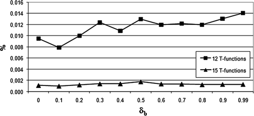
Finally, it is worth mentioning that increasing number of the T-functions in the formula (9) in the case of nodeless FEMT improves the approximate solution. Increasing the number of the T-functions from 12 to 15 decreases the norms of error almost 10 times. The maximum norm (15) for both cases is shown in .
Figure 4. The maximum norm (15) of the temperature field error for 12 and for 15 T-functions approximation in the nodeless FEMT with heat flux regularization and exact ITRs.
6.2. Noisy values of the ITRs
We consider only the first time step. To the exact data describing the ITRs, we have added a random noise with the mean value equal to zero and standard deviation equal to 0.05. Calculations have been performed with the use of the three FEMs and as an energetic minimizing term only the functional JHF has been applied. The norms (16) and (18) of errors for the noisy data are presented in . The results are much worse than those presented in .
Table 7. δL2 norm of errors of the approximated temperature field as a function of the distance δb from the boundary x = 1 and of errors of the identified temperature at the boundary x = 1 for noisy ITRs.
The noisy ITRs have been next approximated with the linear combination of the T-functions
(19)
The unknown coefficients as, s = 1, 2, …, S, are calculated by minimizing the functional
(20)
where Tik are the noisy values of the ITRs. For the calculation we take S = 18. Norms of the errors of the temperature field approximation with the smoothed ITRs are presented in . The errors are similar to those for the exact data (see ).
Figure 5. Norm (16) of the temperature field error for noisy and smoothed ITRs.
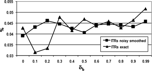
Table 8. δL2 norm of errors of the approximated temperature field as a function of the distance δb from the boundary x = 1 and of errors of the identified temperature at the boundary x = 1 for smoothed ITRs.
7. Conclusions
This article presents new finite element formulations useful for solving IHCPs. An important advantage of the FEM formulation using T-functions in comparison with the conventional FEM results from the property of these functions: they satisfy the governing equation. Thanks to this property, one potential source of inaccuracies is eliminated. The unknown temperature on a part of the boundary has been identified very well even for inaccurate input data.
Compared to the fundamental solution method Citation29,Citation30, which can be considered as a special case of the Trefftz method, the FEMT seems to be less complicated.
The methods presented here are based on the physical properties of the solution. Taking into account the minimization of the temperature jump on the border between elements has been the first factor in improving the approximate solution. Even for the FEMT continuous in the common nodes such an approach smoothes the solution.
Apart from the energetic minimization based on minimizing the heat flux jump on the border between elements, two other kinds of energetic minimization are employed. The results obtained with the use of all the three kinds of energetic minimization are similar. The best results, i.e. the smallest error appears when the functional describing mean-square fitting of the approximate temperature field to the initial, boundary and inner conditions is completed with the functional describing the heat flux inaccuracy between elements.
The nodeless FEMT appears to be most efficient in solving the inverse problems. Moreover, it is easy to improve the accuracy of approximate solution: the more T-functions in the linear combination describing the approximate solution in an element, the better the approximation. However, the more T-functions are taken into account, the worse conditioning of the linear system of algebraic equations for the coefficients of the combination appears. In this case, to solve such an ill-conditioned system of equations, the Tikhonov regularization method may be applied Citation31.
For linear partial differential equations (PDEs) the FEMT seems to be a very good method to solve the inverse problems, because it is not difficult to find T-functions for such linear PDEs. In particular, the nodeless approach and smoothing the inaccurate input data using T-functions are very useful. Numerical results show that this method is effective even for noisy data.
Acknowledgements
This work was carried out in the framework of the research project No. N513 003 32/0541, which was financed by the resources for the development of science in the years 2007–2009.
References
- Reddy, JN, and Gartling, DK, 1994. The Finite Element Method in Heat Transfer and Fluid Dynamics. London: CRC Press; 1994.
- Lewis, RW, Morgan, K, Thomas, HR, and Seetharamu, KN, 1995. The Finite Element Method in Heat Transfer Analysis. New York: John Wiley and Sons; 1995.
- Bergheau, J-M, and Fortunier, FR, 2008. Finite Element Simulation of Heat Transfer. New York: ISTE Ltd and John Wiley & Sons Inc.; 2008.
- Mukaddes, AMM, Shioza, R, and Ogino, M, 2006. Parallel finite element analysis of a non-steady heat conductive problem, Int. J. Theoret. Appl. Mech. 1 (1) (2006), pp. 51–61.
- Ling, X, and Atluri, SN, 2006. Stability analysis for inverse heat conduction problems, Comput. Modeling Eng. Sci. (CMES) 13 (3) (2006), pp. 219–228.
- Grysa, K, Ciałkowski, MJ, and Kamiński, H, 1981. An inverse temperature field in the theory of thermal stresses, Nucl. Eng. Design 64 (2) (1981), pp. 169–184.
- Grysa, K, 1989. On the exact and approximate methods of solving inverse problems of temperature fields. Poznań: Rozprawy, Politechnika Poznańska, 204; 1989, (in Polish).
- Hensel, EC, and Hills, RG, A space marching finite difference algorithm for the one dimensional inverse conduction heat transfer problem, ASME Paper, No. 84-HT-48, 1984.
- Hore, PS, Kruttz, GW, and Schoenhals, RJ, Application of the finite element method to the inverse heat conduction problem, ASME Paper, No. 77-WA/TM-4, 1977.
- Bass, B, 1980. Application of the finite element method to the nonlinear inverse heat conduction problem using Beck's second method, Trans. ASME 102 (1980), pp. 168–176.
- Tikhonov, AN, and Arsenin, VY, 1977. Solution of Ill-posed Problems. Washington, DC: Wiley & Sons; 1977.
- Alifanov, OM, 1994. Inverse Heat Transfer Problems. New York: Springer-Verlag; 1994.
- Jirousek, J, 1978. Basis for development of large finite elements locally satisfying all field equations, Comp. Meth. Appl. Eng. 14 (1978), pp. 65–92.
- Jirousek, J, and Wróblewski, A, 1996. T-elements: State of the art and future trends, Arch. Comp. Meth. Eng. 3 (1996), pp. 323–434.
- Qin, Q-H, 2000. The Trefftz Finite and Boundary Element Method. Southampton: WIT Press; 2000.
- Stein, E, 1973. "Die kombination des modifizierten Treffzschen Verfahrens mit der Methode der Finite Elemente". In: Buck, K, Scharpf, D, Stein, E, and Wunderlich, W, eds. Finite Elemente in der Statik. Berlin: Wilhelm Ernst & Sohn; 1973. pp. 172–185.
- Ruoff, G, 1973. "Die praktische Berechnung der Kopplungsmatrizen bei der Kombination dder Treffzschen Methode und der Methode der Finiten Elemente bei flachen Schalen". In: Buck, K, Scharpf, D, Stein, E, and Wunderlich, W, eds. Finite Elemente in der Statik. Berlin: Wilhelm Ernst & Sohn; 1973. pp. 242–259.
- Wood, WI, and Lewis, RW, 1975. A comparison of time marching schemes for the transient heat conduction equation, Int. J. Numer. Meth. Eng. 9 (1975), pp. 679–689.
- Futakiewicz, S, 1999. "Heat functions method for solving direct and inverse heat conduction problems". In: Ph.D. thesis. Poznań: Politechnika Poznańska; 1999, (in Polish).
- Hożejowski, L, 1999. "Heat polynomials and their applications for solving direct and inverse problems of heat conduction". In: Ph.D. thesis. Kielce: Politechnika Świe¸tokrzyska; 1999, (in Polish).
- Ciałkowski, MJ, and Fra¸ckowiak, A, 2001. Solution of the stationary 2D inverse heat conduction problem by Trefftz method, J. Thermal Sci. 11 (2) (2001), pp. 148–162.
- Ciałkowski, MJ, 2001. New type of basic functions of FEM in application to solution of inverse heat conduction problem, J. Thermal Sci. 11 (2) (2001), pp. 163–171.
- Ciałkowski, MJ, Fra¸ckowiak, A, and Grysa, K, 2007. Solution of a stationary inverse heat conduction problem by means of Trefftz non-continuous method, Int. J. Heat Mass Transfer 50 (11–12) (2007), pp. 2170–2181.
- Sladek, J, Sladek, V, and Hon, YC, 2006. Inverse heat conduction problems by meshless local Petrov–Galerkin method, Eng. Anal. Boundary Elements 30 (2006), pp. 650–661.
- Ciałkowski, MJ, Fra¸ckowiak, A, and Grysa, K, 2007. Physical regularization for inverse problems of stationary heat conduction, J. Inv. Ill-Posed Problems 15 (4) (2007), pp. 347–364.
- Grysa, K, 2003. Heat polynomials and their applications, Arch. Thermodynamics 24 (2) (2003), pp. 107–124.
- Macia¸g, A, and Wauer, J, 2005. Wave polynomials for solving different types of two-dimensional wave equations, Comput. Assisted Mech. Eng. Sci. 12 (2005), pp. 87–102.
- Macia¸g, A, 2007. Wave polynomials in elasticity problems, Eng. Trans. 55 (2) (2007), pp. 129–153.
- Hon, YC, and Wei, T, 2004. A fundamental solution method for inverse heat conduction problem, Eng. Anal. Boundary Elements 28 (2004), pp. 489–495.
- Hon, YC, and Wei, T, 2005. The method of fundamental solutions for solving multidimensional inverse heat conduction problems, Comput. Modeling Eng. Sci. (CMES) 7 (2005), pp. 119–132.
- Huang, CH, and Chen, CW, 1998. A boundary-element-based inverse problem of estimating boundary conditions in an irregular domain with statistical analysis, Numerical Heat Transfer, Part B 33 (1998), pp. 251–268.