Combining spatial support information and shape-based method for tomographic imaging inside a microwave cylindrical scanner

Abstract

A nonlinear inverse scattering problem is solved to retrieve the permittivity maps inside a microwave cylindrical scanner of circular cross-section. In this article, we show how we can improve this minimization scheme by taking advantage of several a priori pieces of information. In particular, a global representation based on a Zernike basis expansion is introduced in order to restrain the class of solutions to functions which have circular spatial support, as is the case with the encountered geometrical configuration. The level-set function formalism is also exploited as the targets are known to be homogeneous by parts. We will show how we can combine the spatial support information and the binary nature of the scatterer, with limited changes of the inversion algorithm. Both synthetic and experimental results will be presented in order to highlight the importance of combining all the pieces of available information.

Keywords:

• level-set functions
• inverse scattering
• nonlinear optimization
• Zernike polynomial
• finite element method
• microwave imaging

AMS Subject Classifications::

• 78A46
• 78A45
• 78M10
• 78M50
• 49K20
• 90C52
• 49Q10
• 41A30
• 33C50

1. Introduction

In the field of inverse scattering, it is well known that all of the available a priori information is greatly needed in order to aid the convergence of the solution scheme towards the desired solution. The available pieces of information can be of several natures, based on the geometrical configuration at hand, the mathematical properties of the various operators which are involved in the scattering process, on assumptions made on the characteristics of the target, etc. In the present case, we want to combine several types of a priori information and incorporate them in the most efficient way in the inversion algorithm. At the same time, we would like to provide a scheme where the modifications of the algorithm are minimal with respect to the various introductions of pieces of information.

The first type of a priori information is related to the envisaged configuration. Indeed, we are currently constructing a microwave circular scanner which consists of a cylindrical column of circular cross-section, surrounded by a ring of antennas. The target is necessarily placed inside the cylindrical column, and the measurements are performed both in reflexion and in transmission, therefore providing a so-called complete configuration. The only piece of information at hand is that the target is included inside a region of circular cross-section. This is the type of low-level piece of a priori information that must be implemented inside the inversion algorithm. One easy way is just to restrain the investigation area to such a circular zone, but it is not sufficient to ensure that the target will have a circular spatial support. A better way consists of projecting the target profile onto a set of basis functions which are all defined on the unit disk. Amongst the available basis functions, the Zernike polynomials are good candidates, due to their orthogonality properties. Apart from the fact that they incorporate in a simple manner the information related to the support, they also provide a global representation of the permittivity profile. The added value is that it enables the number of unknown parameters to be drastically reduced.

The reduction of the number of unknowns is of great importance with respect to the mathematical properties of the radiation operator. Indeed, it has been shown that the radiation operator has the same behaviour as a low-pass filter 1,2. It means that the measured scattered field will have a limited spectrum and, even if the target has a complex shape with details lower than half the wavelength, it will not be possible to retrieve the exact features of the target profile without an additional amount of information. Due to the limited number of independent measurements, there is a limited number of parameters that can be used to represent the permittivity profile 3. Therefore, using a local representation of the unknown is pointless and it is preferable to use a global representation with a limited number of unknown coefficients that can be adequately controlled. By doing so, it is possible to avoid local minima and instabilities. The nice feature of the Zernike polynomials relies on the fact that the first terms correspond to smooth features as the higher terms provide refined spatial details on the scatterer profile. By playing with the number of terms in the Zernike summation, it is possible to remove or add details in the reconstructed maps.

The other a priori piece of information at hand is the fact that the investigated scatterers are necessarily homogeneous and of known permittivity. The level-set function formalism has proved to be one of the most suitable representations to describe the shape of an homogeneous region. In particular, it can handle any kind of topological changes in a very simple manner, such as merging or splitting. This level-set function approach has now been widely used in various domains 4–7 going from inverse scattering to image segmentation. The goal is now to combine the previous a priori piece of information with the level-set function formalism. Several attempts have been made to provide a level-set function description based on a reduced number of coefficients. For example, the contour of the level-set function has been represented in terms of global basis functions such as B-splines 8,9 or spherical harmonics in 3D configurations 10. Unfortunately, this type of representation is not suitable for the forward finite element code that we have implemented and which is based on a volume integral formalism and not on a surface integral formalism. In the present case, it is more appropriate to introduce a global representation for the level-set function itself. Traditionally, the level-set function is represented in terms of a piecewise-constant approximation, the number of unknowns being nothing but the number of pixels. Multi-scaling approach combined with local polynomial interpolation techniques can be used to restrain the number of unknown parameters 11, but this cannot incorporate the piece of information related to the circular shape of the support. Radial basis functions 12 or B-spline interpolation 13 have also been proposed in image segmentation. The problem in that case is to define a suitable algorithm for the control points.

In the present work, we propose to model the level-set function as a continuous parametric function, expressed in the Zernike polynomial basis in order to combine both the limited circular spatial support piece of information and the limited number of degrees of freedom. Moreover, in order to avoid solving the Hamilton–Jacobi equation 14 which controls the deformation of the level-set function during the iterative process, we adopt a mollified version of the Heaviside function 15 in order to work with differentiable functionals. With such an approach, it is still possible to use the Polak–Ribiere scheme which has been first developed in order to retrieve the maps of permittivity profile inside the cylindrical cavity 16.

This article is organized as follows. Section 2 presents the microwave scanner configuration and the forward problem formulation. Section 3 describes the classical Polak–Ribiere scheme which has been developed in order to retrieve continuous maps of permittivity profile inside the cylindrical cavity. In Section 4, the mollified level-set function formalism is introduced together with the slight changes that must be provided to the standard scheme in order to take into account such a piece of a priori information. In Section 5, the restriction on the circular shape of the investigation area is introduced through the Zernike polynomial expansion. This global basis representation is derived either for the permittivity profile, regardless of the homogeneous nature of the scatterer, or for the level-set profile taking this time into account the binary aspect of the permittivity profile. The slight changes provided to the minimization algorithm are also highlighted. Results of reconstructions are presented in Section 6. We have compared the behaviour of the four schemes: without any a priori information, with support information only, with binary information only and with support and binary information together. A purely synthetic configuration is considered first. Results obtained with experimentally acquired scattered fields are also discussed. Conclusions are given in Section 7.

2. Configuration description

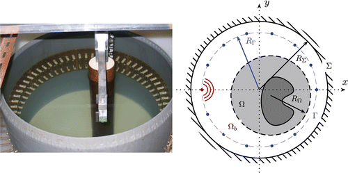
The configuration which is considered here corresponds to the microwave scanner currently under construction at Institut Fresnel. This scanner is made of a cylindrical cavity entirely filled with water. It is enclosed by a metal casing Σ at radius R_Σ = 29.5 cm. This system contains an array of 64 biconical antennas acting as emitters or receivers, and working at a fixed frequency of 434 MHz (Figure 1). These antennas are placed in the same horizontal plane, on a circle Γ of slightly smaller radius than the casing (R_Γ = 27.6 cm) and are adapted to radiate within water. A target is positioned inside the tank and the field scattered by such an obstacle is measured for each couple of emitter–receiver antennas, therefore obtaining a matrix of 64 × 63 measurements. A computer controls the network analyser as well as the multiplexer and stores the measured data.

Figure 1. Picture and cross-section of the microwave scanner measurement set-up presently developed at Institut Fresnel.

Such an environment is presently modelled by solving the Helmholtz equation at the cross-section of interest. It is assumed that both the sample and the sources are infinite along the scanner axis. Therefore, the propagation problem can be solved as a two-dimensional E scalar field problem (transverse magnetic case). Taking into account a time dependence in exp(−iωt), the z-component of the electric field for a given emitter with strength satisfies the following set of equations: (1) where k₀ is the vacuum wave number, and corresponds to the relative permittivity of the target Ω, and ϵ_r,b to the relative permittivity of the embedding liquid Ω_b. The field is the total field which corresponds to the summation of the incident field , measured when there is no target inside the cylinder, and of the scattered field , which corresponds to the field radiated by the currents induced inside the target.

A finite element model is applied to the weak form of the Helmholtz equation (1). The electrical field component is expanded onto linear P₁ basis functions 17. A free unstructured mesh generator 18 is used to discretize the whole domain. The sparse system is solved thanks to the sequential direct sparse solver SuperLu 19 with a very small computational time. Typically, for a first-order triangular mesh with 45,000 nodes, and for the 64 emitting antennas, the run time is about 6 s on a standard PC.

3. Inversion algorithm with no a priori information

When no a priori piece of information is available on the unknown target, the inverse scattering problem is stated as finding the permittivity distribution inside the entire cylinder. Such a problem is traditionally solved by recasting it into a minimization problem with the definition of a discrepancy criterion 𝒥 (2) where corresponds to the scattered field measured by the emitters placed at positions , s = 1, …, N_s, on the probing line Γ. In order to retrieve a permittivity map which matches the measured dataset, the cost functional 𝒥(ϵ_r) must be minimized taking into account the constraints which are provided by Equation (1). It can be shown that the gradient of the cost functional is given by (3) where is the so-called adjoint field which satisfies Equation (1) with a correctly defined field source , where correspond to the receivers positions for a given emitter position.

Taking advantage of the closed-form expression of the gradient, a Polak–Ribiere conjugate-gradient scheme is implemented 20. A sequence of permittivity profiles are then reconstructed based on the following updating scheme: (4) where the descent direction d⁽ⁿ⁾ is given by (5) where ⟨· ∣ ·⟩_Ω represents the inner product defined on L²(Ω) and g⁽ⁿ⁾ is the extension of the gradient of the cost functional on the entire domain (6) The coefficient α⁽ⁿ⁾ is computed using the closed-form solution of the minimum of the following approximated cost functional: (7) where is an approximation at first order of with satisfying the following set of equations: (8)

4. Mollified level-set function formalism

As it is well known, inverse scattering problems are severely ill-posed. Therefore, it is of great interest to take benefit of all available pieces of a priori information, in particular to restrain the class of admissible solutions. Here, we want to take into account the fact that the considered targets are homogeneous and of known permittivity . This means that the unknown is no more the permittivity map, but the shape and location of the various scatterers which are positioned inside the tank.

Significant work exists now on the retrieval of binary obstacles. The level-set function representation has proved to be one of the most suitable representations when no additional topological information is available, such as connexity. This level-set function approach has now widely been used in various applications 5–7. It consists of defining the domain Ω by using a level-set function φ such that (9) The cost functional can now be written as (10)

The next step is to describe the deformation process that the level-set function is going to follow during the minimization scheme. If we derive, according to a fictitious time t which corresponds to the evolution of the iterative scheme, the zero-th level contour of φ, we get 7 (11) where and . In this Hamilton–Jacobi-type equation, the velocity with whom the boundaries of the level-set function are evolving is necessarily linked to the derivative of the cost functional 𝒥.

Unfortunately, such a Hamilton–Jacobi equation is not so easy to solve numerically. When the underlying meshing is performed on a regular grid, a well-known numerical scheme has been proposed 14 and is easily implementable. When the meshing is unstructured, as it is the case with our finite element formalism, it turns out to be more complex. In previous work 21, we have implemented the numerical scheme proposed in 22 which is designed specifically for unstructured meshes. Here, we prefer to avoid solving the Hamilton–Jacobi equation and try to follow as much as possible the Polak–Ribiere scheme described in the previous section. This implies the computation of the derivative of the cost functional 𝒥 with respect to φ. In order to make everything differentiable, a mollified version of the shape description is introduced. The permittivity profile is then expressed as (12) where the mollified Heaviside function H_η and its derivative δ_η are defined by 15 (13) with a mollifying parameter η which controls the size of the transition area of the Heaviside function.

By using the chain rule derivation, we obtain (14) This expression can be seen as the projection of the gradient onto the boundary of the zero-th level of the level-set function. The standard Polak–Ribiere scheme can now be applied by defining the updated level-set function φ, at step n, with (15) and d⁽ⁿ⁾ still follows Equation (5) just replacing g⁽ⁿ⁾ with (16) With such an approach, introducing the homogeneous nature of the scatterers is easily performed with limited changes in the minimization scheme implementation.

5. Zernike polynomials formalism

An additional piece of a priori information can be added to the inversion scheme. Indeed, the targets are known to be positioned inside a tank of circular cross-section. Therefore, the investigation area is necessarily bounded and is of circular shape. It is then of interest to represent the unknowns with functions which have the same circular spatial support. The Zernike polynomials have been selected as they correspond to a set of orthogonal functions for the unitary disk. The Zernike polynomials are expressed 23 in cylindrical coordinates , with respect to the centre of the investigation domain, by (17) where the radial component is defined by (18) where m ≥ 0, l ∈ are integers, m ≥ |l| and m − |l| is even.

We define by ‘order’ of the Zernike polynomials the maximal order achieved by the radial component polynomial, i.e. a representation of order 4 implies that polynomials up to ρ⁴ will participate in the representation of the unknown. The Zernike polynomials behaviour can be interpreted as follows: when the order of the polynomial is increasing, the associated curve presents more and more oscillations with respect to the radial direction. Low orders will correspond to smooth functions while high orders will provide fastly varying functions.

5.1. Projecting the permittivity profile

When there is no a priori information on the nature of the scatterer, such a Zernike representation can be used to represent the permittivity map. In that case, the unknowns are the coefficients such that (19) Using the chain rule derivation and the fact that the Zernike polynomials form an orthogonal basis, we obtain (20) Therefore, in the previous Polak–Ribiere conjugate gradient scheme, the gradient g⁽ⁿ⁾ of Equation (6) is now replaced by the following relationship: (21) The rest of the iterative scheme remains identical, both for the estimation of d⁽ⁿ⁾ and for the computation of α⁽ⁿ⁾.

5.2. Projecting the level-set function

If the scatterer is known to be homogeneous, it is more interesting to expand the level-set function itself. In that case, the unknowns are the coefficients such that (22) Using again the chain rule derivation, we obtain (23) In the previous Polak–Ribiere conjugate gradient scheme, the gradient g⁽ⁿ⁾ of Equation (16) is now replaced by the following relationship: (24) The rest of the iterative scheme remains identical, both for the estimation of d⁽ⁿ⁾ and for the computation of α⁽ⁿ⁾.

5.3. Available information

By using a global representation of the unknowns on a suitably chosen family of basis functions, we have been able to introduce spatial support information in the inversion scheme. The second advantage associated to this representation is to reduce the number of unknowns. Indeed, instead of having as many unknowns as pixels, there are now as many unknowns as coefficients (resp. ) if the permittivity profile (resp. the level-set function) is projected onto the basis functions set. Instead of 10,000 unknowns, there are now 144 unknowns for a Zernike polynomials representation of order 10. It is even possible to find out a correspondence between the number of degrees of freedom 1,2 and the number of coefficients that can be correctly retrieved in the present configuration 24,25. This is also a way to regularize the inversion scheme by restraining the number of unknowns in the minimization process.

6. Numerical and experimental results

In the previous sections, four different ways of resolving the inverse scattering problem have been introduced: no a priori information when searching for ϵ_r with Equation (6), homogeneous scatterer when searching for φ with Equation (16), circular investigation domain and reduced number of unknowns when searching for with Equation (21), and finally homogeneous scatterer with circular investigation domain and reduced number of unknowns when searching for with Equation (24). The four algorithms will be compared and validated using both synthetic data and experimental data.

6.1. Initial guess and stopping criterion

All the iterative sequences start from the same initial estimate, that is . If the level-set function formalism is employed, the level-set function is initialized using the permittivity plot obtained at the first iteration, which provides nothing but the back-propagated profile. The level-set function is then defined with (25) where δϵ is a cut-off which enables to select at the first iteration the points which are part of the scatterers and the points which are in water. A cut-off of δϵ = 0.2 has been taken. The mollifying parameter η is set to 0.1. The rest of the iterative scheme then follows, only considering the level-set function as the unknown.

All the iterative sequences are stopped when either the number of iterations gets over 100 or when the cost functional 𝒥 is reaching a plateau. To detect such a plateau at iteration n_max, the following criterion is used: (26) with n_window = 5 and tol = 10⁻². The stopping criterion is based on the log-scale description of the cost functional as the plateau is much more visible on such a representation.

6.2. Synthetic dataset

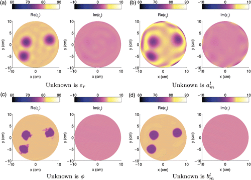
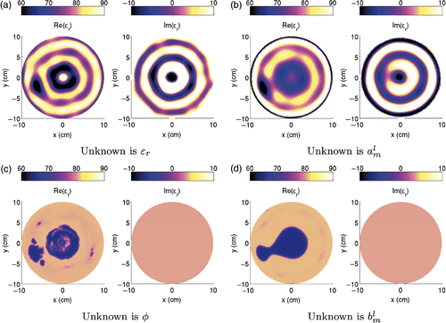
In the considered synthetic configuration, the embedding liquid is assumed to be water with a permittivity of ϵ_r,b = 81 + 3j. Three tubes of radius r = λ_b/4 are placed within the tank. All of them have a permittivity of . The exact permittivity profile is plotted in Figure 2. In order to avoid an inverse crime, the forward problem is modelled with a finer grid than the inverse problem grid. As the experimental dataset will be inverted in the next section, no noise has been introduced in the synthetic case. The 64 × 64 scattered field matrix is taken as input for the four algorithms and the obtained results are plotted in Figure 3 when the order of Zernike polynomials is 10. As expected, due to the low-pass filter nature of the radiation operator, the permittivity profile obtained using Equation (6) is smoothed (Figure 3a). Such a smoothing effect is also present when using Equation (21), as shown in Figure 3(b), and is even enhanced by the fact that not all the orders of the Zernike polynomials are taken into account, but the expansion is truncated at the order 10. Adding information on the binary nature of the scatterer with Equation (16) definitively improves the result, as shown in Figure 3(c). Nevertheless, some spurious oscillations are present due to the numerical noise in the dataset. Equation (24) enables both binary information and Zernike representation to be combined and it provides excellent features, as shown in Figure 3(d). Indeed, the previous oscillations are removed by the smoothing effect of the Zernike polynomials.

Figure 2. (Available in colour online). Exact positioning of the three targets inside the tank in the synthetic configuration. Only the inner circular part of the tank with a radius of 10 cm is plotted.

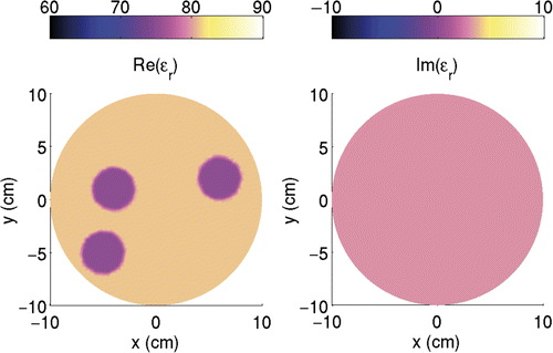
Figure 3. (Available in colour online). Real and imaginary permittivity profiles reconstructed at the end of the four iterative schemes. The results are obtained using the synthetic dataset starting with an initial estimate having the permittivity of the background. Only the inner circular part of the tank with a radius of 10 cm is plotted.

6.3. Experimental dataset

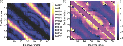
Let us now consider an experimental dataset. Two plastic tubes, filled with a given liquid, are placed inside the tank. The plastic container of the tubes is assumed to be thin enough that it can be neglected in the modelling part. Using liquids ensures that the targets are homogeneous. Moreover, we can a posteriori control the permittivity of the liquid thanks to an open-ended coaxial probe directly connected to the network analyser. The measured water permittivity has been found out to be ϵ_r,b = 81 + 3.5j. The two tubes are filled in with a mixture of 30% of ethanol and 70% of water 26, and the measured permittivity is . In Figure 4, one can see the amplitude and phase of the scattered field matrix. Again, the order of the Zernike polynomials have been stopped at 10.

Figure 4. (Available in colour online). (a) Amplitude and (b) phase of the measured scattered field for each pair of emitter and receiver, when two tubes filled with a mixture of ethanol and water are positioned inside the water tank. The points which are too close to the emitting antenna are excluded.

The final reconstructed images are presented in Figure 5. Due to the experimental errors, the reconstruction obtained without a priori information is noisy with large oscillations. The imaginary part reaches negative values which are not physically acceptable (Figure 5a). Using the Zernike representation for the permittivity profile smooths out slightly the images, but the result is still unsatisfactory (Figure 5b). The introduction of the level-set function is also a good way for constraining the imaginary part and the target shape is more clearly distinguishable (Figure 5c). There are some spots from place to place in a similar manner as in Figure 3c. Finally, combining all a priori information, as in Figure 5(d), provides a very accurate and stable permittivity profile. Unfortunately, the two tubes which were correctly separated in Figure 5(c) are now connected. This is due to the smoothing effect of the Zernike polynomials.

Figure 5. (Available in colour online). Real and imaginary permittivity profiles reconstructed at the end of the four iterative schemes. The results are obtained using the experimental dataset, with an initial estimate having the permittivity of the background. Only the inner circular part of the tank with a radius of 10 cm is plotted.

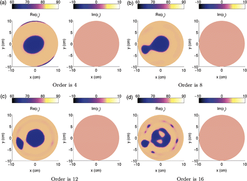
The next step is to vary the order of the Zernike polynomials. As stated before, low orders correspond to small radial oscillations as high orders provide fast radial variations. The reconstructed profiles obtained for various Zernike polynomials order are plotted in Figure 6. From the reconstructed images, it is clearly visible that the low orders smooth out the profiles. The best reconstruction is provided when the order of the Zernike polynomials is 12 as the separation between the two tubes is visible. Let us point out that the distance between the two tubes is of the order of λ_b/5. When the order increases again, oscillations appear and the image gets closer to Figure 5(c). Indeed, there are more and more coefficients to account for the noise components which are present in the measured signal. With the present set-up, the signal to noise ratio is around 15 dB, and part of the current experimental work is to improve this signal to noise ratio.

Figure 6. (Available in colour online). Real and imaginary permittivity profiles reconstructed at the end of the level-set function represented with Zernike polynomials. Several orders of Zernike polynomials are used to limit the number of unknown coefficients . The results are obtained using the experimental dataset, with an initial estimate having the permittivity of the background. Only the inner circular part of the tank with a radius 10 cm is plotted.

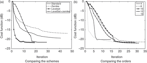
The cost functional behaviour is plotted for the various cases envisaged here (Figure 7). Each time, the cost functional has reached a plateau. The level-set function formalism clearly improves the data fitting, meaning that using an homogeneous assumption for the unknown scatterer is indeed a good option. In terms of Zernike polynomials order, if the order is too low, the measurements are not properly fitted as the solution is much too constrained. Nevertheless, in all cases, there exists a threshold below which the cost functional does not decrease, which corresponds to the level of noise that is present in the measured field.

Figure 7. Evolution of the cost functional along the iterations. (a) The four schemes are compared. (b) The combination of the level-set function formalism and the Zernike polynomials representation is performed for various order of the Zernike polynomials. The dataset corresponds to the measured scattered field.

7. Conclusions

We have presented herein several ways of incorporating pieces of a priori information in order to compensate for the ill-posedness of the inverse scattering problem. First, we have introduced in a simple manner a global representation for the unknowns instead of looking for the value of the permittivity profile in each cell. This was performed using a representation in terms of Zernike polynomials expansion. By doing so, we have divided the number of unknowns by a factor of 50. The benefit is also to take into account the cylindrical shape of the investigation domain and to limit the number of unknown coefficients to retrieve. Second, we have introduced in a very simple manner the homogeneous nature of the targets. This was performed thanks to a representation in terms of a mollified level-set function formalism. Finally, the two pieces of a priori information are combined to provide a mollified level-set function represented in terms of Zernike polynomials.

We have shown that the associated modifications which have been introduced in the standard minimization scheme are small, as only the gradient of the cost functional changes from one scheme to the other one. The behaviour and performance of each scheme have been compared both on synthetic data and experimental data. The configuration which has been studied corresponds to the experimental set-up currently under test at Institut Fresnel. We have shown that the combination of the two pieces of a priori information provides the best reconstructions, which are very robust with respect to noise. This points out the good behaviour and the interest of such a regularization scheme.

In future works, the extension of such an approach to targets which are homogeneous by parts is envisaged 27,28. It would also be of interest to estimate simultaneously the geometrical properties of the target and their homogeneous by parts complex dielectric values 29,30. Concerning the Zernike polynomials, associated work has shown that the number of unknown coefficients to retrieve can be estimated from the measured data spectrum and the signal-to-noise ratio 25. It would also be of interest to investigate a multi-level methodology for determining the best order during the reconstruction process. At the same time, we are working on a three-dimensional modelling code to simulate the exact environment of the microwave circular scanner in a proper way. The issue will be to find a set of basis functions whose spatial support has the shape of a circular cylinder.

Acknowledgements

This work was supported in part by ANR ‘Jeunes Chercheurs’ grant JCJC06-141021 and by INTAS grant 06-1000017-8909. The authors would like to thank the referees for their constructive comments.

References

- Bucci, OM, Crocco, L, and Isernia, T, 1999. Improving the reconstruction capabilities in inverse scattering problems by exploitation of close-proximity setups, J. Opt. Soc. Am. A 16 (1999), pp. 1788–1798.
- Bucci, OM, and Isernia, T, 1997. Electromagnetic inverse scattering: Retrievable information and measurement strategies, Radio Sci. 32 (1997), pp. 2123–2138.
- Isernia, T, Pascazio, V, and Pierri, R, 1997. A nonlinear estimation method in tomographic imaging, IEEE Trans. Geosci. Remote Sens. 35 (1997), pp. 910–923.
- Burger, M, and Osher, SJ, 2005. A survey on level set methods for inverse problems and optimal design, Eur. J. Appl. Math. 16 (2005), pp. 263–301.
- Dorn, O, and Lesselier, D, 2006. Level set methods for inverse scattering, Inverse Probl. 22 (2006), pp. R67–R131.
- Litman, A, Lesselier, D, and Santosa, F, 1998. Reconstruction of a two-dimensional binary obstacles by controlled evolution of a level-set, Inverse Probl. 14 (1998), pp. 685–706.
- Santosa, F, 1996. A level-set approach for inverse problems involving obstacles, ESAIM: Control, Optim. Calculus Variations 1 (1996), pp. 17–33.
- Miller, EL, Kilmer, M, and Rappaport, C, 2000. A new shape-based method for object localization and characterization from scattered field data, IEEE Trans. Geosci. Remote Sensing 38 (2000), pp. 1682–1696.
- Naik, N, Eriksson, J, de Groen, P, and Sahli, H, 2008. A nonlinear iterative reconstruction and analysis approach to shape-based approximate electromagnetic tomography, IEEE Trans. Geosci. Remote Sensing 46 (2008), pp. 1558–1574.
- Zachoropoulos, A, Arridge, S, Dorn, O, Kolehmainen, V, and Sikora, J, 2006. Three-dimensional reconstruction of shape and piecewise constant region values for optical tomography using spherical harmonic parameterization and a boundary element method, Inverse Probl. 22 (2006), pp. 1509–1532.
- Berre, I, Lien, M, and Mannseth, T, 2007. A level-set corrector to an adaptative multiscale permeability prediction, Comput. Geosci. 11 (2007), pp. 27–42.
- Gelas, A, Bernard, O, Friboulet, D, and Prost, R, 2007. Compactly supported radial basis functions based collocation method for level-set evolution in image segmentation, IEEE Trans. Image Process. 16 (2007), pp. 1873–1887.
- Bernard, O, Friboulet, D, Thevenaz, P, and Unser, M, 2008. Variational B-spline level-set method for fast image segmentation, IEEE Int. Symp. Biomed. Imaging (2008), pp. 177–180.
- Osher, S, and Sethian, JA, 1988. Fronts propagating with curvature-dependent speed: Algorithms based on Hamilton–Jacobi formulations, J. Comput. Phys. 79 (1988), pp. 12–49.
- Vese, L, and Chan, T, 2002. A multiphase level-set framework for image segmentation using the Mumford and Shah model, Int. J. Comp. Vision 50 (2002), pp. 271–293.
- Lencrerot, R, Litman, A, Tortel, H, and Geffrin, JM, 2007. A microwave imaging circular setup for soil moisture information, IEEE Int. Symp. Geosci. Remote Sensing (2007), pp. 4394–4397.
- Jin, J, 2002. The Finite Element Method in Electromagnetics. New York: Willey-Interscience; 2002.
- Geuzaine, C, and Remacle, J-F, 2007. GMSH Reference Manual: A three-dimensional finite element mesh generator with built-in pre- and post-processing facilities (2007), Available at http://www.geuz.org/gmsh.
- Demmel, JW, Eisenstat, SC, Gilbert, JR, Li, XS, and Liu, JWH, 1999. A supernodal approach to sparse partial pivoting, SIAM J. Matrix Anal. Appl. 20 (1999), pp. 720–755.
- Nocedal, J, and Wright, SJ, 2006. Numerical Optimization. Berlin: Springer; 2006.
- Cmielewski, O, Tortel, H, Litman, A, and Saillard, M, 2007. A two-step procedure for characterizing obstacles under a rough surface, IEEE Trans. Geosci. Remote Sensing 45 (2007), pp. 185–200.
- Abgrall, R, 1996. Numerical discretization of the first-order Hamilton–Jacobi equations on triangular meshes, Comm. Pure Apl. Math. 49 (1996), pp. 1339–1373.
- Born, M, and Wolf, E, 1959. Principles of Optics. Oxford: Pergamon Press; 1959.
- Crocco, L, and Litman, A, 2009. On embedded microwave imaging systems: Retrievable information and design guidelines, Inverse Probl. 25 (6) (2009), p. 065001.
- Lencrerot, R, Litman, A, Tortel, H, and Geffrin, JM, 2009. Imposing Zernike representation for imaging two-dimensional targets, Inverse Probl. 25 (2009), p. 035012.
- Chaudhari, A, Shankarwar, A, Arbad, B, and Mehrotra, S, 2004. Dielectric relaxation in glycine–water and glycine–ethanol–water solutions using time domain reflectometry, J. Sol. Chem. 33 (2004), pp. 313–322.
- DeCezaro, A, Leitão, A, and Tai, XC, 2009. On multiple level-set regularization methods for inverse problems, Inverse Probl. 25 (2009), p. 035004.
- Litman, A, 2005. Reconstruction by level-sets of n-ary scattering obstacles, Inverse Probl. 21 (2005), pp. S131–S152.
- Dorn, O, and Villegas, R, 2008. History matching of petroleum reservoirs using a level set technique, Inverse Probl. 24 (2008), p. 035015.
- Tanushev, NM, and Vese, LA, 2007. A piecewise-constant binary model for electrical impedance tomography, Inverse Probl. Imaging 1 (2007), pp. 423–435.