Semi-analytic inversion method for the determination of elastoplastic properties of power hardening materials from limited torsional experiment

Abstract

An inverse problem related to the determination of elastoplastic properties of a beam is considered within J₂ deformation theory. A new fast algorithm is proposed for the identification of elastoplastic properties of engineering materials. This algorithm is based on finding the three main parameters of the unknown curve g(ξ²) (plasticity function), namely, the elasticity limit , the modulus of rigidity G and the strain hardening exponent κ. The advantage of this algorithm is that only two values of measured output data are required for the reconstruction of the unknown function g(ξ²). Note that all parameterization algorithms use numerous torsional experiments as necessary data for the determination of only some part of the unknown stress–strain curve. Numerical examples related to applicability and high accuracy of the proposed approach are presented for the cases of noise free and noise data.

Keywords:

• torsional rigidity
• power-law materials
• measured data
• elastoplastic deflections
• parameterization

1. Introduction

The present study deals with an inversion analysis and algorithms for the determination of elastoplastic properties of a beam from a limited number of torsional experiments. Many analytical, computational and experimental studies have already been presented in the scientific literature, especially when small amounts of twisting are reversible, and the beam returns to its original shape after releasing the twisting force. This is called the elastic behaviour. The classic elastic torsion problems have been well-studied in the literature 1–3. However the elastoplastic behaviour of torsional creep is less well-known and it has received relatively little attention in the mathematical, as well as the engineering, literature. An elastoplastic analysis for the torsion of anisotropic bars, using the finite element method and modified Hellinger–Reissner variational principle, has been presented in 4. A numerical study of elastoplastic torsion, based on the finite difference approach to the governing differential equation, has been given in 5. The theory of space curved beams with arbitrary cross-sections, with associated finite element formulation, is implemented in 6 for three-dimensional beams with elastoplastic material behaviour. A rigid-plastic finite element analysis for the torsion of circular, square and rectangular bar sections, related to metal forming, has been presented in 7. The mathematical model of torsional creep within the J₂ deformation theory has been given in 8. In this model one seeks the solution u(x) (deflection function) of the following nonlinear boundary value problem: (1) Here Ω ≔ (0, l₁) × (0, l₂), l₁, l₂ > 0, denotes the cross-section of a bar, and it is assumed to be in ℝ², with piecewise smooth boundary ∂Ω; ϕ is the angle of twist per unit length, g = g(ξ²), ξ² = |∇u|², is defined as the plasticity function and satisfies the following conditions 8–10: (2) For many engineering materials, the function g(ξ²) has the following form 11,12: (3) which corresponds to the Ramberg–Osgood curve σ_i = σ₀(e_i/e₀)^κ. Here κ ∈ (0, 1) is the strain hardening exponent, G > 0 is the shift modulus of rigidity and is an elasticity limit. The value κ = 1 corresponds to pure elastic materials: .

Note that experimental and numerical results related to solutions of basic problems, in particular, spherical indentation problems, show that when stressing is nearly proportional, the new plasticity models predict qualitatively similar behaviour to the J₂ flow and deformation theories 11. Comparing all the plasticity models used for spherical indentation, it has been shown in 13,14 that J₂ deformation theory is used rather than flow theory because it is not only easier to implement numerically, but also it gives essentially identical predictions to the flow theory, when stressing is nearly proportional (simple loading). Taking into account these circumstances, the J₂ deformation theory of plasticity is used here as a physical model. Within the range of this theory, the plasticity function (3) describes the elastoplastic properties of a wide class of engineering materials 11–15. Evidently, this function satisfies all conditions (2). When , the beam is said to be undergoing plastic deformation, so large amounts of twisting can cause the beam to be permanently deformed. In the pure elastic case, g(ξ²) = 3G, where G = E/(1 + ν), and E > 0 is the elasticity modulus. The Poisson coefficient ν ∈ (0, 0.5) is assumed to be known, and it is usually assumed to be ν = 0.3.

Let u = u(x), x = (x₁, x₂) ∈ Ω ⊂ ℝ², be the solution of the nonlinear boundary value problem (1). Then the theoretical value of the torque (or torsional rigidity) is defined as follows 8–10: (4)

In this article, within the range of J₂ deformation theory of nonlinear elasticity, the inverse problem of determining the unknown coefficient g = g(ξ²) in the nonlinear equation (1) from experimentally given discrete values 𝒯_i ≔ 𝒯(ϕ_i) of the torque (or torsional rigidity) is considered. These discrete values are assumed to be given during the quasi-static process of torsion, generated by the angle of twist ϕ_i ∈ [ϕ_*, ϕ*]. Therefore, in the considered physical model the quasi-static process of torsion is simulated by the monotone increasing values 0 < ϕ_* = ϕ₁ < ϕ₂ < ··· < ϕ_M = ϕ* of the angle of twist. Hence the torque 𝒯 ≔ 𝒯(ϕ), whose theoretical value is defined by (4), will be considered as a function of the angle ϕ > 0 (Figure 1). Thus the inverse problem can be formulated as the problem of determining the pair of functions (u(x), g(ξ²)) from the following nonlocal nonlinear identification problem: (5) Here 𝒯_i ≔ 𝒯(ϕ_i) are the measured values of the torque, (measured output data) corresponding to the angles and M > 1 is the number of measurements.

Figure 1. The geometry of the torsion.

In this context, for a given function g(ξ²), satisfying conditions (2), the nonlinear problem (1) will be referred to be as the Dirichlet problem.

The aim of this study is to propose a fast algorithm for the reconstruction of the plasticity function g(ξ²), defined by (3), from only two values of measured output data 𝒯(ϕ₀) and 𝒯(ϕ₁), ϕ₀ < ϕ₁, where the parameter ϕ₀ > 0 corresponds to pure elastic torsion.

The inverse problem (5) has been first considered in 10.

This article is organized as follows. In Section 2 the direct and inverse problems are analysed. In Section 3 a brief description of the parameterization algorithm and ill-posedness of the inverse problem is discussed. The new fast algorithm is described in Section 4. Numerical experiments with noise free and noise data, and also a comparative analysis with parameterization algorithm, are discussed in Section 5. In Section 6 some conclusions are presented.

2. An analysis of the direct and inverse problems: ill-posedness

For the numerical solution of the direct problem (1), we will use the variational approach. This approach is based on the monotone potential operator theory applied to nonlinear elliptic boundary value problems 9. For this aim we define the weak solution of the nonlinear direct problem (1) as follows: (6) where the functionals a(u; v, w) and l(v) are defined as follows: (7) The potential of this problem is defined to be the functional Π(u) = J(u) − l(u), where is the potential of the nonlinear operator Au ≔ −∇.(g(|∇u|²)∇u). For the linearization of the nonlinear variational problem (6), the monotone iteration scheme introduced in 9 is used: (8) Then the potential of the linearized problem (8) is defined by the following functional: (9) The function is defined to be an approximate solution of the direct problem. Substituting (8) in (9) and taking into account (7) we can derive the potential for the linearized direct problem (8) via the torque (10) According to Lemma 1 9, the sequence of potentials {Π(u⁽ⁿ⁾)} is a monotone decreasing one. Since this sequence is also bounded below, it converges. The rate of convergence of the sequence of approximate solutions {u⁽ⁿ⁾} via the potential Π(uⁿ) has been estimated in 9: The error estimate can be given via the torque by using formula (10): For the numerical solution of the linearized direct problem (8), the following finite-difference scheme is used: where is the piecewise uniform mesh with steps h_m = l_m/(N_m − 1), m = 1, 2. Here v_i,j ≔ u⁽ⁿ⁾(x_1,i, x_2j) are the nodal values of the approximate solution u⁽ⁿ⁾(x) (nth iteration). The coefficients are defined as follows:

Now consider the inverse problem for determining the unknown coefficient g = g(ξ²) in the nonlinear elliptic equation (1) from the experimentally given curve 𝒯(ϕ). Let 𝒢 be the set of admissible coefficients g(ξ²) satisfying conditions (2). Denote by u(x, g; ϕ) the solution of the direct problem (1) for a given g ∈ 𝒢 and ϕ ∈ [ϕ_*, ϕ*], ϕ_* > 0. Then the inverse problem (5) can be reformulated as a solution of the following nonlinear functional equation: (11) Based on the definition (4) we define the input–output map T[·]: 𝒢 ↦ T from the class of admissible coefficients 𝒢 to the class of output functions T(ϕ) ∈ T. Then the inverse problem can be reformulated in terms of input–output mapping as follows: (12) This shows that the inverse problem with the given measured output data 𝒯(ϕ) ∈ T can be reduced to the solution of the nonlinear operator equation (12) with an experimentally given right-hand side 𝒯, or to inverting the input–output map T[·]: 𝒢 ↦ T.

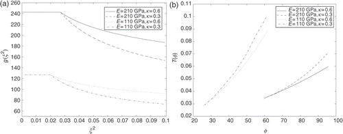
Note that the inverse problem for determining the plasticity function g = g(ξ²) from an experimentally given torque function 𝒯 = 𝒯(ϕ) is a severely ill-posed problem, which means that small changes in the function 𝒯(ϕ) ∈ T may lead to large deviations in the plasticity function g(ξ²) ∈ 𝒢 (see 16). This phenomenon is illustrated in Figure 2 for rigid and soft materials: very close torque curves (b) may correspond to different plasticity functions with κ = 0.6 and κ = 0.3 (a), especially for small elastoplastic deformations.

Figure 2. Plasticity functions for rigid and soft materials, and their corresponding torques.

On the other hand, in practice, the measured output data 𝒯 = 𝒯(ϕ) may only be given with some measurement error, which means that the exact fulfilment of the equality in (11) is not possible. Hence, one needs to introduce the auxiliary (cost) functional (13) and consider the following minimization problem: (14) A solution of the minimization problem (14) is defined to be a quasi-solution of the inverse problem (5). Based on compactness of the set of admissible coefficients 𝒢 in the Sobolev space H¹[ξ_*, ξ*] (see 17), and the continuity of the cost functional (13), the existence of solution of the minimization problem (14) has been proved in 18.

3. Parameterization and divergence of the algorithm

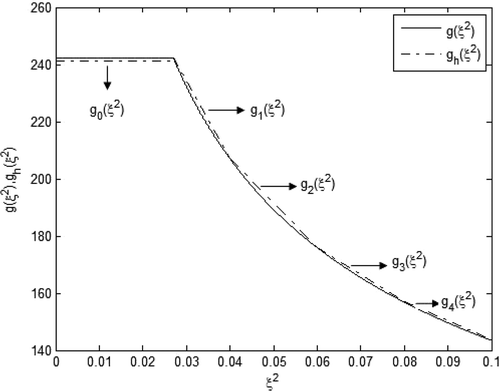
The parameterization algorithm is based on the discretization of the unknown curve (3), by a piecewise linear continuous curve g_h(ξ²), which has the form 18,19 (Figure 3): (15)

Figure 3. The parameterization scheme.

Each discrete parameter , which means maximal value of the stress intensity, , characterizes the mth plastic (for m = 0, elastic) torsional state of a bar. This state is given by the value ϕ_m ∈ [ϕ_*, ϕ*] of the angle of twist. As a result of this parameterization, the discrete analogue of the inverse problem can be formulated as the problem of determining the vector (β₀, β₁, …, β_M) from the experimentally given data (T₀, T₁, …, T_M). The parameter is assumed to be the state discretization parameter.

The unknown parameters β_m > 0 need to be determined step by step by using measured output data 𝒯_m, which corresponds to the discrete values ϕ_m of the angle of twist. In the pure elastic case, the input–output map is an antitone one, as it was proved in 18. This means G₁ > G₂ implies that T[G₁] < T[G₂] ∀G₁, G₂ ∈ 𝒢. This circumstance was taken into account in the algorithm for the determination of unknown parameter β₀ = 3G, i.e. the elasticity modulus G > 0. Assuming that ⟨ϕ₀, 𝒯₀⟩ is a given measured output data corresponding to the pure elastic case, we propose here the following algorithm for the determination the unknown elasticity modulus G = β₀/3.

Algorithm 1

(i) Choose iterations G⁽¹⁾, G⁽²⁾, satisfying the conditions (16)

(ii) use the next iteration G⁽³⁾ = (G⁽¹⁾ + G⁽²⁾)/2, and calculate the theoretical value of the torque T_h[G⁽³⁾] by (4);

(iii) determine the next iteration, using conditions (16):

(iv) calculate the residual |T_h[G⁽³⁾] − 𝒯₀|;

(v) if |T_h[G⁽³⁾] − 𝒯₀| < ϵ_T, then β₀ = G⁽³⁾. Otherwise, continue the steps (ii)–(iv);

(vi) repeat the process until the fulfilment of the stopping condition (17)

The calculated value G_h ≔ G⁽ⁿ⁾ is assumed to be an approximate value of the elasticity modulus G > 0. The parameter ϵ_T > 0 is defined to be of a given accuracy for an approximate solution G_h = G⁽ⁿ⁾ of the inverse problem in the pure elastic torsion.

Having found the elasticity modulus E and the elasticity limit , we may construct similar algorithm for the plastic torsion case. This algorithm can be applied for each mth plastic torsion case, for determination of the slopes β_m > 0, . The parameterization scheme (15) shows that the functional (13) needs to be minimized for each , which means the unknown parameters β_m need to be determined successively on each mth state (step by step), by increasing the angle parameter Δϕ_m = ϕ_m − ϕ_m−1, m = 1, 2, 3, …, M. The first distinguished feature of scheme (15) is that all previously determined parameters β_k, are included in the mth state due to nonlinearity of the forward problem (1). Subsequently, computational errors are compounded, and as a result, a second noise factor–computational noise factor arises. By increasing the number of states, the influence of this factor increases. 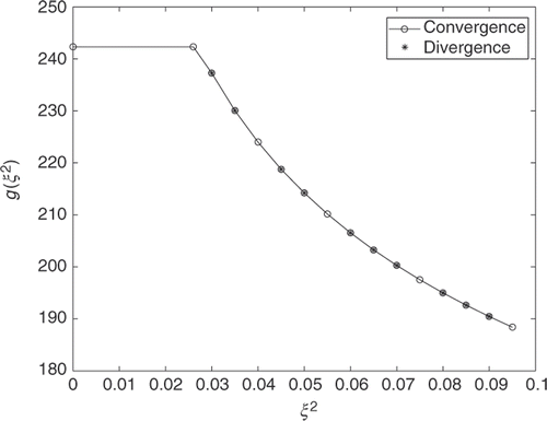Hence for small values of the state discretization parameters , the inverse problem may become unstable at some state. This phenomenon is illustrated in Figure 4, obtained by direct application of scheme (15). Specifically, for small values of the parameters Δϕ_m, which correspond to direct lines in Figure 4 between two neighbouring points and on the plane (ξ², g(ξ²)), the parameterization algorithm diverges immediately at the first plastic state (the first ⋆-point in Figure 4). Also the next increase ()) of the discretization parameter does not lead to the convergence (the second ⋆-point in Figure 4). The subsequent increase of the discretization parameter leads to the convergence of the algorithm (the second ○-point in Figure 4). Further computational experiments show that only the value of the discretization parameter leads to the convergence of the parameterization algorithm, as shown in Figure 4. The measured data 𝒯_m = 𝒯(ϕ_m) for the considered example has been obtained from the quasi-real experiment for a power hardening material with κ = 0.6, , E = 210 GPa, by solving the forward problem (1), and then calculating the theoretical value of the torque (5). Thus, the above results show that the parameterization algorithm may not lead to convergence.

Figure 4. Divergence of the parameterization algorithm.

4. The fast algorithm for identification of the plasticity function for engineering materials

The fast algorithm for the identification of the plasticity function g = g(ξ²), given by (3), consists of three stages.

	Step 1 Determination of unknown rigidity modulus G > 0.
	Step 2 Determination of unknown elasticity limit , and then the corresponding output (measured) data (ϕ1, 𝒯1).
	Step 3 Determination of unknown strain hardening exponent κ ∈ (0, 1).

Since the point on the plasticity curve is the initial point/iteration for all subsequent points, one needs to determine it with high accuracy. For the determination of the unknown elasticity limit we will use the linearity of the direct problem (1). Specifically, let G_h > 0 be the already determined rigidity modulus, and (ϕ₀, 𝒯₀) the corresponding measured output data. We define the new angle of twist as follows: , where δ₀ ∈ (0, 1). Due to the linearity of the direct problem (1) in pure elastic case, the synthetic output data can be generated from the output measured data 𝒯₀ by the formula .

This property will be used in the following algorithm of determining of the unknown elasticity limit .

Algorithm 2

(i) Choose the iteration , satisfying the condition ;

(ii) use the synthetic output data , , and apply Algorithm 1 to find ;

(iii) calculate the relative error δG⁽¹⁾ = |(G_h − G⁽¹⁾)/G_h|;

(iv) (a) if δG⁽¹⁾ < ϵ_G, use the next iteration ; (b) if δG⁽¹⁾ > ϵ_G, use the next iteration ;

(v)use the synthetic output data , , and repeat the items (ii)–(iii);

(vi)repeat the process until the fulfilment of the following conditions: Here , and the functions , are the solutions of the corresponding direct problems.

The value is assumed to be an approximate value of the elasticity limit . The pair , corresponding to this value of the elasticity output is defined to be the output (measured) data for last pure elastic deformation case.

Having found the values of the rigidity modulus G_h > 0 and the elasticity limit , we can determine the unknown hardening exponent κ ∈ (0, 1) using only one (single) measured data, corresponding to plastic deformations. This is due to the explicit form , of the plasticity function, given by (3). Let (ϕ₁, 𝒯₁) be the given noise free output measured data for plastic deformation case, i.e. . We use the above parameterization algorithm to reconstruct the unknown parameter β₁ in (18) This parameter is determined by Algorithm 1. Having the parameters and β₁, we substitute the function g_h(ξ²), given by (18), in the direct problem, and then solving it we can calculate the maximum value of the deformation intensity ξ². Since the point needs to be on the plasticity curve g = g(ξ²), from the explicit form (13) of the plasticity function we obtain the following equation: for the determination of the approximate value κ_h of the unknown strain hardening exponent κ ∈ (0, 1). This equation implies that . Hence the parameter κ_h is defined as follows: (19) As the denominator of the above fraction shows, the value ξ_1h cannot be chosen close to ξ_0h (otherwise, this is one of the reasons of the ill-posedness of the considered inverse problem). This means that, the angle step needs to be chosen large enough for the well-posedness of formula (19). This conclusion is also asserted by the computational experiments below.

Formula (19) permits one to define analytically the approximate value κ_h of the strain hardening parameter κ ∈ (0, 1) for power hardening materials. Hence the proposed approach can be defined as a semi-analytic inversion method. The most distinguished feature of this method is not only its usefulness in practice and simplicity, but also that it uses only two values of measured output data and (ϕ₁, 𝒯₁) for the reconstruction of the plasticity function g(ξ²) given by (3). In addition, while the parameterization algorithm may reconstruct a part of the plasticity curve, depending on the number M > 1 of measured output data, the fast algorithm determines the whole plasticity curve, defined in (0, (ξ*)²).

5. Numerical experiments with noise free and noise data

The following two types, ; , of rigid and soft materials, with different hardening parameters (κ = 0.2 and κ = 0.6) were used in implementation of the proposed algorithm. Noise free synthetic data for these materials were generated by solving the direct problem (1) with this data, and subsequently numerical calculating the theoretical values of torque, given by the integral (4).

In the first series of computational experiments Algorithm 1 is implemented for the determination of the shift modulus G = E/2(1 + ν) for rigid (E = 210 GPa) and soft (E = 110 GPa) engineering materials. In all the computational experiments below the Poisson coefficient is assumed to be known (ν = 0.3). The algorithm for reconstruction of the approximate values of the shift modulus G_h > 0 was applied for the following three values ϵ_T = 10⁻²; 10⁻³; 10⁻⁴ of the stopping parameter. The corresponding relative errors δG_h = |G − G_h|/G were found as δG_h = 10⁻²; 10⁻³; 10⁻⁴, respectively. This shows that the relative error δG_h decreases proportionally by decreasing the stopping parameter ϵ_T > 0. Evidently, this is due to linearity of the considered problem for the pure elastic case. The number n of iterations in the implementation of Algorithm 1 was obtained 6, 7. Taking into account these results in subsequent computational experiments, the stopping parameter ϵ_T > 0 for the cost functional (13) was set to be ϵ_T = 10⁻⁴. In this case an approximate value of the shift modulus G = 80.77 of the rigid material was found as G_h = 80.74.

At the second stage, Algorithm 2 was implemented for the determination of the unknown elasticity limit for rigid and soft materials, with the already found approximate values of the shift modulus G. With the first input data G_h = 80.74 for the rigid material, the reconstructed elasticity limit was , while computed from the direct problem solution, with the same input data, the elasticity limit was . Similar results are obtained for the soft material, with G = 42.30.

From the natural experiments point of view, it is interesting to define also the level of accuracy in the measured values ϕ_i of the angle of twist, corresponding to the value ϵ_T = 10⁻⁴ of the stopping parameter. With this aim, the linear direct problem (g(ξ²) = 3G, G = 80.77) was solved which gave two values ϕ₁, ϕ₂, with |ϕ₁ − ϕ₂| = 0.12. The absolute error was found, ϵ_T ≔|T[g](ϕ₁) − T[g](ϕ₂)| = 0.9 × 10⁻⁴. Therefore, in the case of pure elastic deformations, the above accepted value ϵ_T = 10⁻⁴ of the stopping parameter corresponds to the absolute error δϕ = 10⁻¹ in the measured values of the angle of twist, which can be defined as an accuracy of the torsional experiment for pure elastic case. Almost the same results were obtained for the soft material with G = 42.30. Specifically, the above value, ϵ_T = 0.9 × 10⁻⁴, corresponds to the absolute error |ϕ₁ − ϕ₂| = 3.5 × 10⁻¹ in the measured values of the angle of twist.

As was stated above, the point on the plasticity curve g = g(ξ²) plays an important role in the reconstruction of the unknown plasticity function, as an initial point/iteration for subsequent iterations, and hence needs to determined with high accuracy. Since this accuracy also depends on the angle step , the reconstruction of the parameter β₁ in (18) was performed for three increasing values 3.5, 7.0, 12.0 of the angle step Δϕ₁. The approximate values of the parameter κ and the corresponding relative errors (δκ = |κ − κ_h|/κ) obtained by formula (19) are presented in Table 1. The optimal angle step is Δϕ₁ = 12.0, as Table 1 shows. For all three cases the plasticity functions reconstructed the fast algorithm, as shown in Figure 5. To compare these results, the parameterization algorithm was also applied for the determination of the plasticity function g(ξ²), by taking four values of synthetic measured output data (ϕ_i, 𝒯_i), and the optimal angle step Δϕ₁ = 12.0. The reconstructed plasticity function is plotted in the same figure by the dotted line under the solid line (exact solution). The results show that the fast algorithm gives a better reconstruction using a minimal number of measured data.

Figure 5. The reconstructed curves g_h(ξ²) for different values of the angle step for rigid material (noise free data).

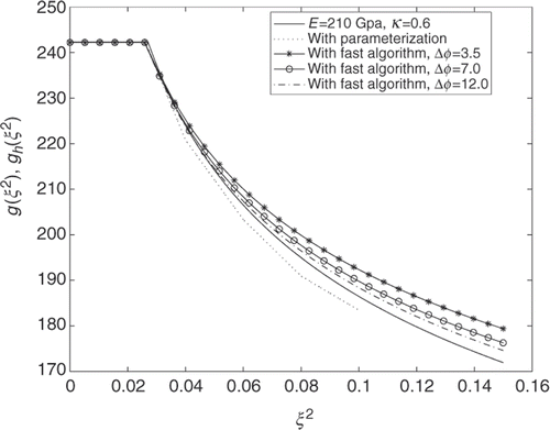
Table 1. Angle steps Δϕ₁ and corresponding errors δκ in the reconstruction of the parameter κ.

Δϕ1	κh	δκ
3.5	0.656	9.3 × 10^−2
7.0	0.636	6.0 × 10^−2
12.0	0.625	4.1 × 10^−2

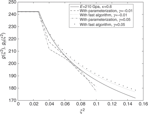
In practice, the torque 𝒯 can only be given with some measurement error γ, i.e. with noise data 𝒯_γ = 𝒯 + γ𝒯. In computational material sciences these errors are usually assumed to be from ±1% to ±5%. Two types of noise levels–lower noise with γ = ±0.01 and higher noise with γ = ±0.05–are used in computational experiments. Results are presented in Figure 6. For noise factor γ = ±0.01, the approximate value of the main unknown parameter κ was found as κ_h = 0.641, while for noise factor γ = ±0.05, respectively, this value was found as κ_h = 0.650. The relative errors are δκ = 6.8 × 10⁻² and δκ = 8.3 × 10⁻², correspondingly. Although some increase in the relative error is observed for the higher noise level, the obtained results show that this error remains at the same order, 10⁻². Low sensitivity of the fast algorithm with respect to noise factor shows its well-posedness.

Figure 6. The reconstructed curves g_h(ξ²), with noise data and Δϕ = 12.0 for rigid material.

To compare the proposed algorithm with the parameterization algorithm in the case of noise data, the latter was implemented in the presence of four values of synthetic measured output data (ϕ_i, 𝒯_i), , where the first data again corresponds to pure elastic deformation. The reconstructed piecewise linear curves corresponding to the noise data 𝒯_γ with the noise levels γ = −0.01 and γ = 0.05, are plotted in Figure 6. Note that the above four values of measured data are being sufficient to define the piecewise linear curve only in the interval (0, ξ²) = (0, 0.1). Comparing in this interval and the numerical results obtained by these two algorithms, we can conclude that the relative error δκ corresponding to the fast algorithm is less than the relative error corresponding to the parameterization algorithm. Therefore, using the minimal number of values of measured data, the fast algorithm gives a better reconstruction, even in the interval , corresponding to small elastoplastic deformations.

Note that similar results obtained for soft engineering materials were almost the same, in the sense of accuracy and relative errors.

6. Conclusions

A new inversion algorithm for identifying the elastoplastic properties of engineering materials described by the Ramberg–Osgood curve is proposed. The first distinguishing feature of this algorithm is that it uses only two values of data (ϕ_i, 𝒯_i), i = 0, 1, relating the angle of twist, ϕ_i, with the corresponding value of torque 𝒯_i. These measured value data are generated during the quasi-static process of torsion given by the angles ϕ₀ and ϕ₁. In addition, the first data (ϕ₀, 𝒯₀) corresponds to the pure elastic case and the second data (ϕ₁, 𝒯₁) to the plastic torsion case. The proposed fast algorithm is based on the reconstruction of the triple (G, ξ₀, κ) (shift modulus, elasticity limit and strain hardening exponent), sequentially, which defines one-to-one the plasticity function g(ξ²) (or the Ramberg–Osgood curve) for power hardening engineering materials. The second distinguishing feature of this algorithm is its well-posedness. The numerical results for the different engineering materials show that the present algorithm allows the reconstruction of elastoplastic parameters with high accuracy for acceptable noise levels.

Acknowledgements

This article is based upon the work supported by the Scientific and Technological Research Council of Turkey (TUBITAK) under grant No. 108T332. This work is also supported by the Izmir University Research Fund, through the International Research Projects Grant. The authors also thank the referees whose comments and suggestions substantially improved the revision of this article.

References

- Timoshenko, SP, and Goodyear, JN, 1970. Theory of Elasticity. New York: McGraw Hill; 1970.
- O'Leary, D, 2004. Elastoplastic torsion: Twist and stress, Comput. Sci. Eng. 6 (2004), pp. 74–76.
- Bertola, V, and Cafaro, E, 2005. Geometric approach to laminar convection, J. Thermophys. Heat Transfer 19 (4) (2005), pp. 581–583.
- Boonlualohr, P, and Valliappan, S, 1976. Elastoplastic torsion of anisotropic bars, J. Eng. Mech. 102 (1976), pp. 995–1008.
- Bland, JA, 1993. Implementation of an algorithm for elastoplastic torsion, Adv. Eng. Software 17 (1993), pp. 61–68.
- Gruttmann, F, Sauer, R, and Wagner, W, 2000. Theory and numerics of three-dimensional beams with elastoplastic material behaviour, Int. J. Numer. Meth. Eng. 48 (2000), pp. 1675–1702.
- Park, Y-B, and Yang, D-Y, 2007. Analysis of torsional deformation by rigid-plastic finite element method using recurrent boundary conditions, J. Mater. Process. Technol. 182 (2007), pp. 303–311.
- Kachanov, LM, 1961. "The Theory of Creep (Gosizdat Fizmatlit, Moscow, 1960)". In: Problem of Continuum Mechanics. Vol. 202. Philadelphia: SIAM; 1961.
- Hasanov, A, 2008. Convexity argument for monotone potential operators and its application, Nonlinear Anal. Theory Methods Appl. 41 (2008), pp. 907–919.
- Mamedov, A, 1995. An inverse problem related to the determination of elastoplastic properties of a cylindrical bar, Int. J. Non-Linear Mech. 30 (1995), pp. 23–32.
- Wei, Y, and Hutchinson, JW, 2003. Hardness trends in micron scale indentation, J. Mech. Phys. Solids 51 (2003), pp. 2037–2056.
- Cao, YP, and Lu, J, 2004. A new method to extract the plastic properties of metal materials from an instrumented spherical indentation loading curve, Acta Mater. 52 (2004), pp. 4023–4032.
- Budiansky, B, 1959. A reassessment of deformation theories of plasticity, J. Appl. Mech. 26 (1959), pp. 259–264.
- Fleck, NA, and Hutchinson, JW, 2001. A reformulation of strain gradient plasticity, J. Mech. Phys. Solids 49 (2001), pp. 2245–2271.
- Rikards, R, Flores, A, Ania, F, Kushnevski, V, and Balta Calleja, FJ, 1998. Numerical experimental method for the identification of plastic properties of polymers from microhardness tests, Comput. Mater. Sci. 11 (1998), pp. 233–244.
- Hasanov, A, and Tatar, S, 2009. Solutions of linear and nonlinear problems related to torsional rigidity of a beam, Comput. Mater. Sci. 45 (2009), pp. 494–498.
- Hasanov, A, 1997. Inverse coefficient problems for monotone potential operators, Inverse Probl. 13 (1997), pp. 1265–1278.
- Hasanov, A, and Erdem, A, 2008. Determination of unknown coefficient in a nonlinear elliptic problem related to the elastoplastic torsion of a bar, IMA J. Appl. Math. 73 (2008), pp. 579–591.
- Hasanov, A, 2007. An inversion method for identification elastoplastic properties from limited spherical indentation measurements, Inverse Probl. Sci. Eng. 15 (6) (2007), pp. 601–627.