Solution of Cauchy problem to stationary heat conduction equation by modified method of elementary balances with interpolation of the solution in physical plane

Abstract

This article presents a solution of stationary direct and inverse problems (Cauchy problem) of cooling a circular ring with the modified method of elementary balances. The idea of the method itself relies on the division of the considered range into elements and interpolation of the solution within the elements with the help of linear combination of base functions. In the vicinity of every mesh node, the control regions are created in which the energy is balanced. The regions include or interpenetrate with each other. The numerical calculation has been carried out with the use of a quadrilateral mesh with four nodes and a triangular mesh with six nodes. The presented solution to the inverse problem with randomly perturbed boundary conditions of the flux and temperature at the outer boundary of the ring with maximal error reaching up to 10% gave very good results. The solution of the inverse problem has been obtained in the sense of singular value decomposition algorithm.

Keywords:

• inverse problem
• the method of elementary balances
• Cauchy problem

1. Introduction

This article will consider the inverse problem of steady heat conduction of Cauchy type. The Cauchy problem for Laplace equation is ill posed in Hadamard sense 1.

In recent years, the Cauchy problem for a two-dimensional Laplace equation has been considered by many authors. The review presented below is limited to papers in which numerical implementation was an essential element of the paper. In 2, the boundary element method was used for numerical implementation of the alternating algorithm proposed by Kozlov et al. 3 for solving the Cauchy problem for the Laplace equation. In the numerical experiment, the authors tested their method for solving a problem in the square region with a known exact solution. The same procedure was used by these authors 4 for the Cauchy problem for anisotropic heat conduction. In 5, authors using Green's formula transformed the Cauchy problem to a Hausdorff moment problem. Two test examples in the unit square region were solved to verify the effectiveness of the proposed method. The similar approach was proposed by Hon and Wei 6, where the moment problem was solved by the Backus–Gilbert algorithm. The Cauchy problem in two connected regions (square domain with square hole) was considered in 7. The authors used two different methods for solving the considered problem. The first one was the finite difference method with the additional use of the Tikhonov regularization. In the second one, the conformal mapping was used to map square region with a square hole to annulus and the solution of the problem was based on the fast Fourier transformation. Both the proposed methods require rather a lot of computations and the obtained results are comparable. In 8, a Cauchy problem with Poisson equation was solved by means of the dual reciprocity method, based on the boundary element method. The authors successfully solved test problems in circular, annular and square regions using Tikhonov regularization. Another successful approach of several test problems was presented in 9, where the author used a linear combination of radial basis functions as an approximate solution and collocated differential equation and boundary conditions by the Kansa method 10. The advantage of the Kansa method in comparison with traditional mesh methods, such as the finite difference method, finite element method, and boundary element method in the solution of the Cauchy problem is its meshless character and the continuity of derivatives of the approximate solution of the required order. The method of fundamental solutions 11 shares similar advantages. Marin 12 examines the application of the method of fundamental solutions (MFSs) 11 to the Cauchy problem for steady heat conduction in two-dimensional functionally graded materials. The author employed the Tikhonov regularization method with the L-curve criterion as the regularization parameter. The problems in one connected region as test examples were considered. The same method was used for a Cauchy problem for anisotropic heat conduction in one connected region 13. Wei et al. 14 also consider the one connected region based on MFSs. The authors presented some interesting numerical experiments with different regularization techniques and different choice of the regularization parameters. The MFSs with condition number analysis for the Cauchy problem was considered in 15. The authors drew a very interesting conclusion that ‘many problems traditionally considered to be ill-conditioned, now can be accurately calculated without difficulty by using the proposed MFS together with analysis of a conditional number without regularization. It is well known that the MFS belongs to a family of Trefftz methods with their characteristic feature – the exact satisfaction of the governing equation. A different kind of Trefftz method is based on T-functions instead F-functions (fundamental solutions) for fundamental solutions. For a Cauchy problem, this version of Trefftz method was considered in 16.

As the review of the available literature shows, the MFSs is the method used most frequently to solve the Cauchy problems due to its numerous advantages essential for this type of issue. The basic advantages of MFS are the continuity of solution and its derivatives of any order, as well as the exact solutions of the heat conduction equation.

For the multiply connected regions in application of MFS, the essential problem is the determination of optimal number of sources and their positions (additional parameters are: number of sources, distance of sources from boundary of region). It leads to an ill-conditioned system of equations and the conditioning decreases with the increasing number of sources. The larger number of sources is needed for a more exact description of the changing of boundary conditions in the Cauchy problem.

In the solution of the inverse problem of ring cooling presented in 18, the method of elementary balances has been applied that is significantly different from the classical approach.

A basis for the method of elementary balances makes the integral equations of energy, momentum, and mass balance. The equations are true for any sub-range included in the considered range. In the case of the method of elementary balances, the free choice of sub-range is delimited to an arbitrarily determined mesh on which the physical values are balanced. Taking into account the method of approximation of the functions representing the solution of the differential equation and its derivatives, the method develops in two main directions 19:

1.	Control volume method (CVM) with the function derivatives approximated with the help of finite differences.
2.	Control volume finite element method (CVFEM) where the function and its derivatives are approximated by differentiation of a function that interpolates the solution of the partial differential equation.

Therefore, in both cases, there are two overlapping meshes. One of them serves for approximating the solution, while on the other the physical values are balanced, e.g. the heat flux in the case of heat transfer problems or momentum in the case of equations of motion. At the same time, it was assumed that physical values, such as heat, mass or momentum flux, flow from one element of the balanced mesh to a neighbouring one in equal amounts. In the first case, the equality is understood in the average-integral sense while in the second one, the distribution of the physical values results from approximation of the solution in an element of the interpolation mesh. The solution is interpolated in a manner similar to the finite element method in the isoparametric space, where continuity of the approximate solution between the mesh elements is ensured and, moreover, the integrals are easily calculated. In the case of higher order interpolation, the transformation of a mesh element to the isoparametric space, the transformation Jacobian may be singular.

The method presented in this article is a generalization of the considerations of 18 and belongs to the class of CVFEM methods. According to the approach applied in 18, the solution on one of the meshes (temperature distribution) has been interpolated based on temperature values in element nodes of one mesh and, afterwards, the heat flux has been balanced based on the solution at the boundaries of another mesh. This way, the idea of approximating the solution within an element by means of interpolation, characteristic for the finite element method has been connected with the idea of balancing the physical values, characteristic for the method of elementary balances. The application of the overlapping meshes with the goal of formulating the solution of the inverse problem of ring cooling gave good results in connection with a low degree of solution interpolation within the element (with four base functions in a quadrilateral element).

Hence, the need arises for more general formulating of the method presented in 18 that converts itself into approximating (interpolating) the solution in a mesh element of any shape for a larger number of mesh nodes. Generalization of the method leads to:

1.

The approximation of the solution to the differential equation in a mesh element in physical space in which the solution is continuous while passing from one element to another. This enables the problems of calculating the integrals for higher order interpolation of the solution within the mesh element to be omitted. The construction of the base functions is based on the idea presented in [20]. These functions have been used for calculation in 18.

2.

Balancing around a common node of several elements, the balancing area being, in general, different from the one where the solution is interpolated (Figures 2 and 3). In particular, the meshes may overlap.

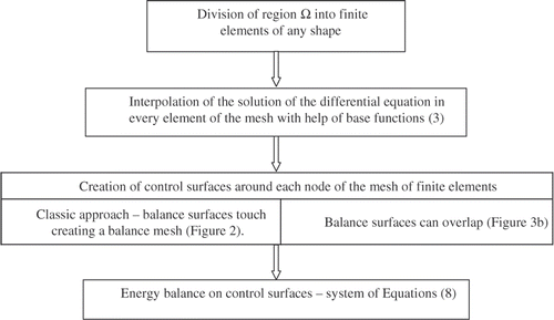
2. Formulation of a modified method of elementary balances (MCVM, modified control volume method)

In the modified method of elementary balances, the domain Ω is divided into sub-domains Ω_n. The unknown solution of the differential equation is interpolated in every element of the domain with the help of base functions. (1)

The base functions ϕ_i are determined as follows: (2) where the points P_j are interpolation nodes belonging to the Ω_n sub-domain. In the case of four nodes of a quadrilateral element or six nodes of a triangular one (Figure 1), the base function ϕ_i is a product of two linear functions [21] (3) where j₁ and j₂ are the numbers of lines connecting the mesh nodes of the element (Table 1), A_jx + B_jy + C_j = 0 being equation of the jth straight line. More general formulation of the interpolation function of such a form in the mesh element is provided by Frąckowiak 19. An important property of the base functions (3) lies in their zeroing at the sides opposite to the P_i node which in consequence leads to the disappearance of some integrals in the calculation process.

Figure 1. Arrangement of six mesh nodes of a triangular element or four nodes in a quadrilateral one.

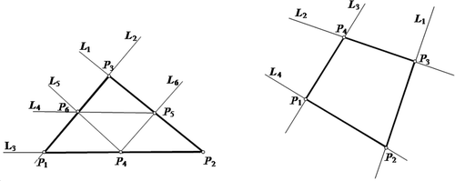
Table 1. The numbers j₁ and j₂ of the straight line for the ith base function.

i	Triangle		Quadrilateral
	j1	j2	j1	j2
1	1	5	1	2
2	2	6	2	3
3	3	4	3	4
4	1	2	4	1
5	2	3
6	3	1

The control surface ∂Σ, on which the energy is balanced, is created around each of the mesh nodes. Figure 2 shows the way of generating the control surface (broken line) for four-node and nine-node elements of a quadrilateral mesh.

Figure 2. Four-node and nine-node elements of a quadrilateral mesh. The solid line denotes an interpolation mesh, while the broken one is for the balance mesh.

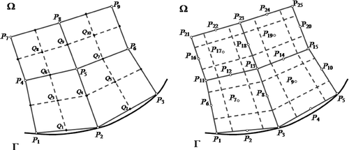
For six-node element of a triangular mesh the shape of the control surface (Figure 3a) becomes more complicated, since in this case the control surface coincides with the mesh lines. This leads to overlapping of control surfaces around various points (Figure 3b).

Figure 3. Six-node element of a triangular mesh; an example of control surface formulation (broken line): (a) polygonal region of balancing around node and (b) circular region of balancing.

For the point P₅∈Ω (Figure 2) the open polygon Q₃Q₄Q₅Q₇Q₉Q₁₀Q₈Q₆Q₃ is a control surface ∂Σ₅, while for the point P₂∈Γ it is the open polygon P₂Q₁Q₃Q₄Q₅Q₂P₂. In the case of a six-node element of a triangular mesh the situation is more complex. Four cases are possible:

1.	P13∈Ω, the control surface is defined by the open polygon P1 P3 P5 P15 P19 P11 P1,
2.	P8∈Ω, the control surface is defined by the open polygon P1 P3 P5 P13 P1,
3.	P3∈Γ, the control surface is defined by the open polygon P3 P5 P13 P1 P3 and
4.	P2∈Γ, the control surface is defined by the open polygon P1 P3 P13 P1.

The example shows that the control surfaces built on a triangular mesh are not disjoint. Energy balance on the control surface for stationary heat conduction equation div(∇T) = 0 performed with the use of the Gauss–Ostrogradski theorem around each point P_i∈Ω leads to the relationship (4) while for the point P_i∈Γ (5) where ∂Σ_i is a control surface around the ith mesh point and Γ_i is part of the outer boundary that coincides with the control surface around the ith point.

Taking into account that the Kirchhoff substitution transforms the non-linear equation div(∇T) = 0 into linear one , we assume λ = 1 for further consideration.

For the point P₅∈Ω (Figure 2), the energy balance is as follows: (6) while in case of P₂∈Γ (7)

The normal derivative in each of the integrals is calculated from an interpolation function that approximates the solution of differential equation within the element

The density of the heat flux q between the points of the Γ boundary is approximated with the help of a linear function

The substitution of the integrals calculated in the manner, into Equations (6) and (7) provides an equation including unknown values of the T(x,y) function in the mesh nodes and the heat flux values at the Γ boundary. The upper index of the base function ϕ is the number of the mesh element.

The similar procedure is applied in the case of the triangular mesh. The energy balance around each of the nodes provides the system of equations (8)

Each of the equations of the system (8) is related to energy balance around the mesh node. The points are located inside the Ω domain (the vector T with index β) or at the Γ boundary (the vectors T and Q with index α). Denote the numbers of outer and inner mesh nodes as n_α and n_β, the number of equations with unknown T_α, Q_α and T_β. It amounts to (2n_α + n_β) of unknowns. Missing T_α and Q_α values are determined from the boundary conditions.

The system of equations (Equation (8)) allows for the elimination of the T_β vector (9) that provides the relationship between temperature and the heat flux at the domain boundary known from the boundary element method (10)

Recapitulating, one can state that in the classical method the balancing is based on consistency of the fluxes between the control domains. In a general case considered here, the balance occurs in mesh around the node, while the control domains may contain each other. Therefore, the present approach to the method of elementary balances is distinguished by the following characteristic features.

1.	In every mesh element, the temperature function is approximated with the help of the interpolation functions (3) (without any constraints imposed on the number of the element nodes).
2.	A control domain, in which the energy is balanced, is created around each of the mesh nodes.

The idea of the method is similar to CVFEM [20], however, the work of Wróblewska et al. 18 and this article indicate important discrepancies between both methods. The differences are related to the interpolation of the solution of the differential equation in finite element and the way the physical values are balanced around the mesh node. The following steps of the modified elementary balance method are shown in Figure 4.

Figure 4. Scheme of generation of system of equations in MCVM.

3. Numerical example

The modified control volume method (MCVM) is applied here to solve the direct and inverse problems of ring cooling. Both problems are formulated identically as in 18.

1.	The direct problem – the third kind boundary conditions are given on the inner and outer ring boundaries (Figure 5), i.e. the heat transfer coefficient α (Biot numbers) are known at the ring boundaries

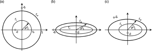
Figure 5. Region Ω: (a) circular ring, (b) elliptical ring, and (c) elliptical ring with displaced boundaries.

(11) (12) where the index o is related to physical values referring to the outer boundary and i to the inner boundary; T_wo and T_wi to the temperature distribution at the ring boundaries.

1.	The inverse problem is formulated by temperature and heat flux density distributions at the outer ring boundary (the Cauchy problem for the Laplace equation).

Example 1: The analytical solution used to compare the calculations performed with this method is expressed by the relationship 1. (13) where T_c = T(1, ϕ), constant C is equal to the amount of heat transferred through the outer boundary of the ring

Boundary conditions of a direct problem for the case of C = 0.5, a = 0.4, T_c = 0.9 and r_o = 0.5 are shown in Figure 6(a), while for an inverse one in Figure 6(b).

Figure 6. Boundary conditions for (a) direct problem (coefficient of heat exchange α on the boundary of the ring) and (b) inverse problem (temperature and density of heat flux on the outer boundary of the ring) in Example 1.

Example 2: Boundary conditions for the circular ring region (Figure 5a) are generated from the formula (14) where C₀ = 0.7, C₁ = −0.1, C₂ = 0.2, . (Figure 7).

Figure 7. Boundary conditions for (a) direct problem (coefficient of heat exchange α on the boundary of the ring) and (b) inverse problem (temperature and density of heat flux on the outer boundary of the ring) in Example 2.

Example 3: Boundary condition for elliptical ring (Figure 5b) boundaries are given by equation are generated from formula (14) for C₀ = 0.7, C₁ = −0.1, C₂ = 0.2 and . (Figure 8).

Figure 8. Boundary conditions for (a) direct problem (coefficient of heat exchange α on the boundary of the ring) and (b) inverse problem (temperature and density of heat flux on the outer boundary of the ring) in Example 3.

Example 4: Boundary conditions for the elliptical ring with variable thickness region (Figure 5c) and boundaries are given by equations: are generated from formula (14) for C₀ = 0.7, C₁ = −0.1, C₂ = 0.2 and . (Figure 9).

Figure 9. Boundary conditions for (a) direct problem (coefficient of heat exchange α on the boundary of the ring) and (b) inverse problem (temperature and density of heat flux on the outer boundary of the ring) in Example 4.

The calculation has been carried out for a six-node element of the triangular mesh and a four-node element of the quadrilateral mesh (Figure 1) for the interpolation of the solution as an element. The parameters of meshes of finite elements used in the particular examples are presented in Table 2. The energy balance around each of the mesh nodes provided in both cases the system of equations (10) that was transformed according to temperature and heat flux separation at the outer and inner ring boundaries for the direct problem (15) and for the inverse problem (16)

Table 2. Parameters of meshes of finite elements used in the numerical calculations.

	Triangular mesh elements			Quadrilateral mesh elements
Example	Number of inner nodes	Number of nodes on the boundary	Number of inner nodes	Number of nodes on the boundary	Number of inner nodes	Number of nodes on the boundary
1	700	200	400	800	200	900
2	3800	400	2000	3600	400	3800
3	1400	400	800	1600	400	1800
4	3800	400	2000	3600	400	3800
Note: The number of nodes on the inner boundary of the ring equals the number of nodes on the outer boundary.

The formula (16) for the inverse problem contains a pseudo-inverse matrix determined with the singular value decomposition (SVD) algorithm.

The algorithm is based on decomposition of a rectangular matrix where and are orthonormal matrices and W is a diagonal matrix, the values of which are square roots of the eigenvalues of the AA^T matrix arranged in a decreasing sequence. The efficiency of the algorithm is related to the f parameter, which may assume values from 1 to 16 (in the case of double-precision computation). Its application is conducive to the condition in which the eigenvalues, for which the condition is met, are converted to zero. The smaller the value of the f parameter, the larger the number of eigenvalues adjusted to zero. In the case of direct problems, its value is not of particular significance. On the other hand, for the inverse problems, the eigenvalues become meaningful and are conducive to the problem regularization.

The results of calculations for the triangular and quadrilateral meshes in case of the inverse problem of ring cooling are shown in Figures 10–13. The plots are made for the known undisturbed temperature and flux values at the outer ring boundary.

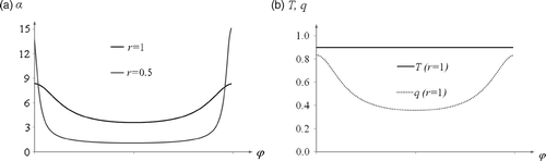
Figure 10. Distribution (a) temperature and (b) density of heat flux on inner boundary of ring for undisturbed data, f = 5 in Example 1.

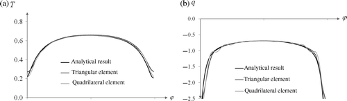
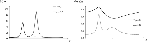
Figure 11. Distribution (a) temperature and (b) density of heat flux on inner boundary of ring for undisturbed data, f = 3 in Example 2.

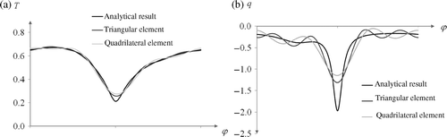
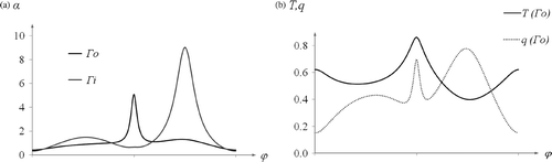
Figure 12. Distributions (a) temperature and b) density of heat flux on inner boundary of ring for undisturbed data, f = 5 for triangular element and f = 3 for quadrilateral element in Example 3.

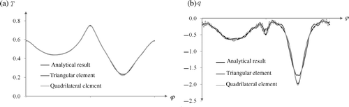
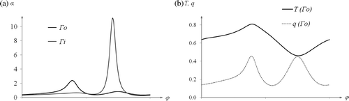
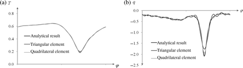
Figure 13. Distribution (a) temperature and (b) density of heat flux on inner boundary of ring for undisturbed data f = 3 in Example 4.

For estimation of both grids, the relative norms 18 have been calculated, which expressed errors of physical value at the ring boundary in comparison with the analytical solution (17)

Boundary conditions of both problems are disturbed with the relative error given by the formula (18) where random is for a pseudo-random number in the range (0,1).

In order to minimize the errors of heat flux and temperature at the boundary, the patterns of these values have been smoothed by means of a linear combination of trigonometric functions 18.

A comparison of the solution errors defined by the norm (17) and disturbed with random error (18) is shown in Tables 3–6 for the temperature and in Tables 7–10 for heat flux density, respectively.

Table 3. Comparison of relative errors in the norm (17) for the temperature with respect to the problem type, the f parameter of the SVD algorithm and the number of base functions m serving for smoothing the disturbed boundary conditions in Example 1.

		Triangular mesh element					Quadrilateral mesh element
Type		The error, εmax (%)					The error, εmax (%)
m	f	0	0.5	1	5	10	0	0.5	1	5	10
The direct problem
		0.24	0.25	0.30	0.76	2.06	0.14	0.16	0.23	0.82	2.14
The inverse problem
	3	1.23	1.66	3.05	11.57	35.95	1.71	1.79	1.83	5.09	10.44
	5	0.7	18.18	30.22			0.33	6.35	10.63	54.85
	8	0.7	12.61	36.37			6.66
	10	0.7	26.31	32.97			6.66
	12	14.8	27.03	99.06			6.66
The inverse problem with smoothed boundary conditions
90	3	1.51	1.56	1.9	4.22	8.6	1.71	1.74	1.81	3.11	5.58
	5	1.12	14.15	24.3			0.33	8.12	13.26	42.55
	8	1.12	13.93	37.38			6.66
	10	1.12	14	31.28			6.66
	12	55.76	59.74	68.05	55.76	55.89	6.66
20	3	1.51	1.52	1.56	1.88	3.52	1.71	1.72	1.73	2.36	3.62
	5	1.13	3.37	6.02	24.61	46.72	0.33	7.49	11.35	35.56
	8	1.13	2.33	3.75	21.8	49.02	0.38	17	27.57
	10	1.13	1.96	3.33	27.81	35.59	0.38	20.68	23.94
12	55.76	55.8	55.8	59.82	65.29	0.38	48.08
4	3	2.9	2.9	2.9	2.9	3.33	2.74	2.74	2.74	2.87	3.46
	5	2.9	2.89	2.9	2.93	3.61	2.74	2.74	2.75	2.81	2.99
	8	2.9	2.89	2.91	2.92	3.08	2.74	2.74	2.74	2.82	2.75
	10	2.9	2.9	2.9	2.96	2.93	2.74	2.74	2.74	2.78	3
	12	55.83	55.82	55.81	55.95	55.79	2.74	2.74	2.74	2.82	3.12

Table 4. Comparison of relative errors in the norm (17) for the temperature with respect to the problem type, the f parameter of the SVD algorithm, and the number of base functions m serving for smoothing the disturbed boundary conditions in Example 2.

		Triangular mesh element					Quadrilateral mesh element
Type		The error, εmax (%)					The error, εmax (%)
m	f	0	0.5	1	5	10	0	0.5	1	5	10
The direct problem
		0.07	0.07	0.07	0.12	0.22	0.01	0.02	0.03	0.09	0.19
The inverse problem
	3	1.08	1.77	4.14	10.75	17.90	1.72	1.74	1.80	3.20	5.84
	5	1.15					0.34	5.15	20.48
The inverse problem with smoothed boundary conditions
90	3	1.51	1.56	1.9	4.22	8.6	1.71	1.74	1.81	3.11	5.58
	5	1.09	1.10	1.23	2.28	5.50	1.72	1.73	1.77	2.45	4.27
	8	1.74	11.95	11.24			0.34	13.69	13.35
20	3	1.10	1.12	1.16	2.07	4.06	1.73	1.74	1.75	1.97	3.09
	5	1.74	4.18	12.25			0.38	6.50	14.55
	8	1.74	6.16	14.81			0.38	6.83	17.76
4	3	3.55	3.55	3.55	3.61	3.60	3.54	3.54	3.54	3.61	3.60
	5	3.55	3.55	3.55	3.58	3.66	3.54	3.54	3.55	3.58	3.65

Table 5. Comparison of relative errors in the norm (17) for the temperature with respect to the problem type, the f parameter of the SVD algorithm, and the number of base functions m serving for smoothing the disturbed boundary conditions in Example 3.

		Triangular mesh element					Quadrilateral mesh element
Type		The error, εmax (%)					The error, εmax (%)
m	f	0	0.5	1	5	10	0	0.5	1	5	10
The direct problem
		0.10	0.09	0.10	0.27	0.30	0.02	0.03	0.07	0.23	0.30
The inverse problem
	3						0.65	0.69	0.83	2.81	4.96
	5	0.30	1.53	2.93	12.47	21.83	0.09	7.31
	8	0.18
The inverse problem with smoothed boundary conditions
90	3						0.65	0.71	0.75	1.91	3.97
	5	0.31	0.61	1.03	5.16		0.17
	8	1.13	4.22	7.71			5.67
20	3						0.88	0.88	0.90	1.41	2.37
	5	0.86	0.93	1.07	2.20	4.05	5.56	5.52	6.80	4.95
	8	2.90	2.69	3.34	6.14	5.22
4	3						6.76	6.76	6.78	6.67	6.97
	5	6.82	6.84	6.84	6.79	6.99	7.23	7.25	7.25	7.20	7.41
	8	6.89	6.88	6.92	6.78	6.73

Table 6. Comparison of relative errors in the norm (17) for the temperature with respect to the problem type, the f parameter of the SVD algorithm, and the number of base functions m serving for smoothing the disturbed boundary conditions in Example 4.

		Triangular mesh element					Quadrilateral mesh element
Type		The error, εmax (%)					The error, εmax (%)
m	f	0	0.5	1	5	10	0	0.5	1	5	10
The direct problem
		0.06	0.06	0.06	0.15	0.19	0.01	0.02	0.04	0.12	0.19
The inverse problem
	3	5.12	5.20	5.35	8.28		1.34	1.37	1.42	3.03	5.28
	5	0.32	3.59	8.69			0.12
	8	1.17					2.35
The inverse problem with smoothed boundary conditions
90	3	5.12	5.12	5.14	5.61	6.59	1.34	1.35	1.38	2.41	3.51
	5	0.33	0.70	1.22	7.41		0.12	9.48	8.51
	8	1.11					2.35
20	3	5.12	5.13	5.10	5.18	5.76	1.34	1.34	1.34	1.68	2.50
	5	0.34	0.71	1.38	5.16		0.59	1.20	3.66	9.74
	8	3.44
4	3	6.58	6.58	6.57	6.61	6.56	4.41	4.41	4.41	4.43	4.43
	5	4.91	4.91	4.91	4.91	4.98	5.82	5.82	5.81	5.80	5.92

Table 7. Comparison of relative errors in the norm (17) for the flux with respect to the problem type, the f parameter of the SVD algorithm and the number of base functions m serving for smoothing the disturbed boundary conditions in Example 1.

		Triangular mesh element					Quadrilateral mesh element
Type		The error, εmax (%)					The error, εmax (%)
m	f	0	0.5	1	5	10	0	0.5	1	5	10
The direct problem
		2.77	3.24	4.03	15.18	28.70	1.55	2.14	3.12	13.82	25.60
The inverse problem
	3	14.44	15.75	22.06	90.10		17.93	18.13	18.18	31.44	62.61
	5	6.40					8.02
	8	6.40
	10	6.40
The inverse problem with smoothed boundary conditions
90	3	14.49	14.71	15.26	20.63	47.92	17.93	18.04	18.20	22.71	33.49
	5	6.51					8.02
	8	6.51
	10	6.51
20	3	14.49	14.51	14.98	16.91	22.24	17.93	17.94	17.99	19.65	25.57
	5	6.79					8.02
	8	6.79	48.19				11.78
	10	6.79	40.01				11.78
4	3	22.61	22.61	22.61	22.68	23.61	22.50	22.50	22.50	22.92	24.84
5	22.61	22.61	22.61	23.00	24.88	22.50	22.50	22.51	22.68	23.44
	8	22.61	22.61	22.61	22.81	23.55	22.50	22.50	22.50	22.71	22.53
	10	22.61	22.62	22.61	22.73	22.65	22.50	22.50	22.50	22.59	23.10

Table 8. Comparison of relative errors in the norm (17) for the flux with respect to the problem type, the f parameter of the SVD algorithm, and the number of base functions m serving for smoothing the disturbed boundary conditions in Example 3.

		Triangular mesh element					Quadrilateral mesh element
Type		The error, εmax (%)					The error, εmax (%)
m	f	0	0.5	1	5	10	0	0.5	1	5	10
The direct problem
		0.58	0.63	0.78	2.81	5.69	0.07	0.27	0.51	2.54	5.37
The inverse problem
	3						17.31	17.29	17.57	27.17	34.05
	5	10.07	35.43				8.24
The inverse problem with smoothed boundary conditions
90	3						17.31	17.67	17.43	21.34	47.46
	5	9.88	16.02	24.55			12.23
20	3						17.61	17.57	17.79	21.54	26.26
	5	18.95	21.42	24.32	50.07
4	3						37.91	37.91	37.93	37.88	37.79
	5	40.48	40.50	40.51	40.50	40.39

Table 9. Comparison of relative errors in the norm (17) for the flux with respect to the problem type, the f parameter of the SVD algorithm, and the number of base functions m serving for smoothing the disturbed boundary conditions in Example 2.

		Triangular mesh element					Quadrilateral mesh element
Type		The error, εmax (%)					The error, εmax (%)
m	f	0	0.5	1	5	10	0	0.5	1	5	10
The direct problem
		0.59	0.68	0.84	2.62	5.39	0.12	0.30	0.56	2.58	5.20
The inverse problem
	3	24.28	30.99				30.71	30.72	30.82	33.02	39.72
	5						12.66
The inverse problem with smoothed boundary conditions
90	3	24.30	24.45	25.21	25.73	57.60	30.71	30.72	30.77	31.42	36.68
	5	66.69					12.66
20	3	24.32	24.37	24.53	31.67	48.62	30.72	30.74	30.75	30.86	34.52
	5	66.70					12.69
4	3	40.17	40.21	40.16	40.85	40.37	40.15	40.19	40.13	40.83	40.35
	5	40.17	40.18	40.19	40.35	39.77	40.15	40.16	40.17	40.33	39.74

Table 10. Comparison of relative errors in the norm (17) for the flux with respect to the problem type, the f parameter of the SVD algorithm, and the number of base functions m serving for smoothing the disturbed boundary conditions in Example 4.

		Triangular mesh element					Quadrilateral mesh element
Type		The error, εmax (%)					The error, εmax (%)
m	f	0	0.5	1	5	10	0	0.5	1	5	10
The direct problem
		0.53	0.59	0.86	2.61	5.26	0.11	0.25	0.59	2.58	5.13
The inverse problem
	3	53.53	53.53	53.50	53.78	54.68	27.38	27.38	27.44	31.23	30.03
	5	11.30					5.45
The inverse problem with smoothed boundary conditions
90	3	53.53	53.53	53.54	53.64	53.76	27.38	27.40	27.38	30.84	32.04
	5	11.30	18.79	29.49			5.48
20	3	53.53	53.53	53.54	53.56	53.52	27.38	27.38	27.49	28.01	29.67
	5	11.88	18.66	36.40			21.35	38.41
4	3	53.98	53.98	53.98	54.00	53.94	47.56	47.56	47.54	47.61	47.50

4. Summary

The Tables 3–10 show that solution of a direct problem with the use of a triangular mesh based on six nodes and a quadrilateral mesh based on four nodes is highly accurate in the sense of the norm (17) with error, ε_max below 5%, i.e. values of the flux and temperature found in the results of the calculation are below 5.5% for temperature, while in case of the flux are below 15%.

The analysis of Figures 10–13 and results presented in Tables 3–10 for the numerical examples 1–4 show a significant conformity of the temperature distribution with the analytical solutions for the regularization parameter on SVD algorithm, f = 3 below 5% for the error of disturbed of data, ε_max ≤ 1%. The heat flux on the inner boundary of the ring shows strong oscillations around the analytical solutions for both types of meshes, which leads to a loss of stability of the solution as the maximal error of disturbed data ε_max increases. This phenomenon is characteristic for the solution of the inverse problem and it is possible to demonstrate that for the Cauchy problem for a circular ring, it is independent for the numerical method of used to solve the problem (an ill-posed problem in Hadamard's sense). A small disturbance in the temperature T(1, ϕ) and heat flux q(1, ϕ) on the boundary Γ_o, lead to a large disturbance of the value of the solution of the Laplace equation on the boundary Γ_i. Lets assume indeed that the disturbances of functions T(1, ϕ) and q(1, ϕ) on the boundary Γ_o are as follows: and we are able to calculate the values of functional of errors of the solution of the Laplace equation at the boundaries Γ_o i Γ_i:

The numerical solution has a form of solution in closed form. By analogy to the above result, it is possible to make the conclusion that the larger the value of parameter f and error ε_max, the larger the value of error of solution.

The calculation results are stable for the small values of the parameter f, which means that the solution of the system of equations (10) was obtained at the borderline of the application of the SVD algorithm. This opens the door to the other direction in research, where the Tichonow regularization is applied to solve that system of equations or it is solved by the iterative solution of sequence of direct problems.

The smoothness of disturbed data has no influence on the value of parameter f, but has only less improvement of the solution of the Cauchy problem for the disturbed data.

The calculation results obtained for the two different cases of energy balancing do not differ much. In the case of the quadrilateral element mesh the control area is generated around the mesh node where the energy balance is performed in a way similar to that used in the classical method of elementary balances (finite volumes), while in the case of a triangular mesh the control areas around different nodes may interpenetrate. This makes a significant difference with respect to the classical method of elementary balances and CVFEM, as it indicates the way of generalization of the method to the meshes of various shapes.

Acknowledgements

The work has been carried out within the framework of the Ministry of Science and Education grant no. 3134/B/T02/2007/33.

References

- Bicadze, AW, 1984. Równania Fizyki Matematycznej. Warszawa: Państwowe Wydawnictwo Naukowe; 1984.
- Lesnic, D, Elliott, L, and Ingham, DB, 1997. An iterative boundary element method for solving numerically the Cauchy problem for the Laplace equation, Eng. Anal. Bound. Elem. 20 (1997), pp. 123–133.
- Kozlov, VA, Maz’ya, VG, and Fomin, AV, 1991. An iterative method for solving the Cauchy problem for elliptic equation, Comput. Math. Math. Phys. 31 (1991), pp. 45–52.
- Mera, NS, Elliott, L, Ingham, DB, and Lesnic, D, 2001. A comparison of boundary element method formulations for steady state anisotropic heat conduction problems, Eng. Anal. Bound. Elem. 25 (2001), pp. 115–128.
- Cheng, J, Hon, YC, Wei, T, and Yamamoto, M, 2001. Numerical computation of a Cauchy problem for Laplace's equation, ZAMM 81 (2001), pp. 665–674.
- Hon, YC, and Wei, T, 2001. Backus–Gilbert algorithm for the Cauchy problem of the Laplace equation, Inverse Probl. 17 (2001), pp. 261–271.
- Berntsson, F, and Elden, L, 2001. Numerical solution of a Cauchy problem for the Laplace equation, Inverse Probl. 17 (2001), pp. 839–853.
- Farcas, A, Elliott, L, Ingham, DB, and Lesnic, D, 2003. The dual reciprocity boundary element method for solving Cauchy problems associated to the Poisson equation, Eng. Anal. Bound. Elem. 27 (2003), pp. 955–962.
- Li, J, 2004. A radial basis meshless method for solving inverse boundary value problems, Commun. Numer. Meth. Eng. 20 (2004), pp. 51–60.
- Kansa, EJ, 1990. Multiquadratics – A scattered data approximation scheme with applications to computational fluid dynamics I, Comput. Math. Appl. 19 (1990), pp. 127–145.
- Fairweather, G, and Karageorghis, A, 1998. The method of fundamental solutions for elliptic boundary value problems, Adv. Computat. Math. 9 (1998), pp. 69–95.
- Marin, L, 2005. Numerical solution of the Cauchy problem for steady-state heat transfer in two-dimensional functionally graded materials, Int. J. Solids Struct. 42 (2005), pp. 4338–4351.
- Jin, B, Zheng, Y, and Marin, L, 2006. The method of fundamental solutions for inverse boundary value problems associated with the steady-state heat conduction in anisotropic media, Int. J. Numer. Methods Eng. 65 (2006), pp. 1865–1891.
- Wei, T, Hon, YC, and Ling, L, 2007. Method of fundamental solutions with regularization techniques for Cauchy problems of elliptic operators, Eng. Anal. Bound. Elem. 31 (2007), pp. 375–385.
- Young, DL, Tsai, CC, Chen, CW, and Fan, CM, 2008. The method of fundamental solutions and condition number analysis for inverse problems of Laplace equation, Int. J. Comput. Math. Appl. 55 (2008), pp. 1189–1200.
- Liu, C-S, 2008. A modified callocation Trefftz method for the inverse Cauchy problem of Laplace equation, Eng. Anal. Bound. Elem. 32 (2008), pp. 778–785.
- Wróblewska, A, Frąckowiak, A, and Ciałkowski, M, 2008. Numerical solution of a direct and inverse stationary problem of heat transfer with a modified method of elementary balances, Arch. Thermodyn. 29 (1) (2008), pp. 1–15.
- Gresho, PM, and Sani, RL, 2000. Incompressible Flow and the Finite Element Method. Vol. 2. John Wiley and Sons, Ltd; 2000.
- Frąckowiak, A, 2008. Base functions of the Finite Element Method and their properties. Funkcje bazowe dla metody elementów skończonych i ich własności, Zeszyty Naukowe Politechniki Poznańskiej 63 (2008), pp. 15–25.