An efficient numerical algorithm for crack reconstruction in elastic media by the circular US scanning

Abstract

In the present work, a direct numerical reconstruction algorithm is proposed, which is applied to the identification of the position and shape of cracks detected in elastic solid samples, in the case when the input data available for the reconstruction is provided by a circular ultrasonic (US) scanner. The US probe gives the far-field back scattered pattern over the full interval of the incident polar angle. The problem is first reduced to a system of basic boundary integral equations. Then the inverse reconstruction problem is formulated as a minimization problem for a certain strongly nonlinear functional. The proposed numerical algorithm is tested on some examples of complex-shaped cracks. Then the influence of the error in the input data on the precision of the reconstruction is studied in detail.

Keywords:

• crack reconstruction
• ultrasonic scanning
• inverse problem
• boundary integral equation
• displacement discontinuity method

1. Introduction

It is well-known in engineering applications that elastic solids with such defects as cracks possess absolutely different mechanical properties when compared with homogeneous ones 1,2. Some standard non-destructive techniques, such as ultrasonic (US) evaluation may be applied to test the mechanical properties of cracked materials (see, e.g. 3,4). In engineering practice the theory of failure plays a key role for evaluation of long-term behaviour of elastic solids working as critical elements in various constructions. In particular, it is very important to know the image (position, characteristic size and shape) of the boundary surface of the defects, and circular US scanning may be used for this purpose. If one can measure the back-scattered far-field diagram for a wide range of the incident angle, say by the echo method, then the problem of the defect identification is reduced to a typical inverse problem. Nowadays, the existing methods seem to be rather efficient qualitatively but not highly precise quantitatively.

Inverse scattering problems are well-developed in the theoretical aspect. If only one type of elastic wave (longitudinal or transverse) plays the key role in wave propagation and diffraction, then as a first approximation the problem can be formulated in frames of a scalar model. Some general aspects of the theory in this case are presented in the literature (see, e.g. 2–4). The basic results are typically concerned with uniqueness 5–9. Unfortunately, less attention is paid to numerical reconstruction algorithms, which is the subject of principal interest for the present authors.

In the present work, we study the two-dimensional inverse problem of linear isotropic elasticity, when both longitudinal and transverse waves take part in the diffraction process. The problem is to restore the true shape of the crack located inside this elastic space. The crack may be of arbitrary shape, and even self-intersecting. It is assumed that the input data for the inverse problem is based on the measured far-field scattering diagram, which can be recorded by a US transducer as a result of the circular scanning in the echo regime at a certain frequency.

Mathematically, the formulation is based upon a system of integral equations holding over the face of the crack. If this boundary face is known then a standard boundary element method (BEM) technique permits the calculation of the far-field scattered pattern. A specific property of the arising system of boundary integral equations (BIE) is that the kernels possess a hyper-singular behaviour. In the case when the boundary of the crack is unknown, the inverse reconstruction problem is to choose such a crack whose scattering diagram coincides with the measured pattern amplitude function versus the angle of incidence. We do not pay attention to fundamental theoretical questions like uniqueness or existence. Instead we propose a certain numerical algorithm which provides a fast real-time reconstruction.

2. Formulation of the problem and basic relations for a single elementary crack

Figure 1 demonstrates the scanning by US sensors which are used to reconstruct the image of a crack located in the elastic solid. The geometry of the crack may be of any complex form, in particular, self-intersecting. The boundary faces of the crack are free of normal and tangential stress. We assume that the far-field amplitude A(α) of the back scattered wave (echo regime) can be measured for a number of directions α of the incident wave.

Figure 1. Far-field US scanning of the unknown crack under reconstruction.

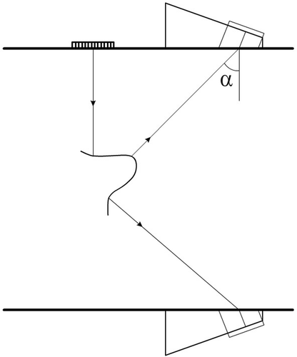
Very often the scanning can be provided for the full circular scattering diagram, i.e. for 0 ≤ α ≤ 2π. This can be arranged either for longitudinal or transverse waves. To be more specific, let us assume that the longitudinal wave is dominant 1. Of course, this does not mean that the problem is scalar, since in the diffraction process both types of elastic waves take part. However, when recording the reflected wave, one keeps only the information about the longitudinal one. Let us assume that the circular frequency is ω, then the dependence upon time e^−iωt is hidden to be not shown in the forthcoming formulae.

Let us assume that the wave process is physically linear and the elastic medium is homogeneous and isotropic. Let us study the basic geometry related to a single crack of arbitrary complex shape located in the unbounded elastic medium (Figure 1). Our goal is, first of all, to calculate analytically the stress–strain field in the medium around the crack.

If we study the two-dimensional plane strain dynamic problem, then the equations of motion, written in a fixed rectangular Cartesian coordinates xy are given by the following system of partial differential equations: (1) where (2) ρ is the mass density, c_p is the longitudinal wave speed, c_s is the transverse wave speed, k_p and k_s are respective wave numbers and quantities {u_x(x, y), u_y(x, y)} denote the components of the displacement vector u.

The components of the stress tensor are given by the following relations: (3)

Considering the structure of the elastic wave field around the full-length crack, we give the solution to this problem following 10–12, in the form of a system of BIE which is called ‘the displacement discontinuity method’. In the dynamical case this can be directly developed with the use of the Fourier transform.

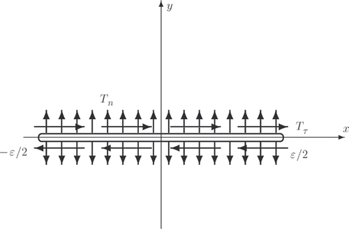
For this aim we study an isolated (elementary) linear crack (Figure 2) placed at the centre of the chosen Cartesian coordinate system. The length of the elementary crack is equal to ϵ which is a small positive quantity, so that the left tip of the crack is (−ϵ/2, 0) and the right one is (ϵ/2, 0). Let us assume that the crack faces are subjected to some (uniform) normal and tangential stresses, T_n and T_τ, and the relative displacement of the crack faces caused by this applied load, along x and y, are respectively, g_x(x) and g_y(x), (|x| ≤ ϵ/2). Then the analytical solution to the problem under consideration can be constructed by using the Fourier transform along the x-axis. Namely, for any function f(x, y) its Fourier transform is denoted by corresponding capital letter, so that the pair of (direct and inverse) Fourier transforms is valid: (4)

Figure 2. An elementary crack in the elastic medium.

Application of the Fourier transform reduces system (2.1) of partial differential equations to a system of ordinary differential equations with constant coefficients (5) where all derivatives are related to variable y.

The characteristic polynomial of this system is (6) since . Equation (2.6) is in fact a biquadratic algebraic equation whose four roots are (7) Here all branching root squares are taken as their arithmetic values, i.e. positive root-square values for positive quantities.

Now one can write the solution to this elementary crack problem constructed separately on the upper (y > 0) and the lower (y < 0) half-planes as a general solution of system (2.5), which according to the radiation condition 2 can be represented in the following form: (8) where A^± = A^±(s) and B^± = B^±(s) are some unknown quantities. It is obvious that these four unknown constants should be defined by satisfying respective boundary conditions. Note that all upper signs are related to the upper half-plane y ≥ 0 and the lower ones to the lower half-plane y ≤ 0.

Let us assume for a while that the ‘opening’ of the crack is known, i.e. both normal g_y(x) and tangential g_x(x) relative displacements of the opposite crack faces are known. Then the boundary conditions over the line y = 0 are continuity of the normal and the tangential stress, and the condition of the known relative displacement over crack faces: (9) where we also assum that the crack faces do not interact with each other.

Relations (2.9) can be rewritten in terms of the Fourier transform of corresponding functions. Available representation for the required stress-tensor components in the Fourier variables can be derived from Equations (2.3) and (2.8): (10) Taking into account representations (2.8) and (2.10), boundary conditions (2.9) can be reduced to the following 4 × 4 system of linear algebraic equations for constants A⁺, B⁺, A⁻, B⁻: (11) which can simply be decomposed to a pair of independent 2 × 2 systems, the first one for quantities A⁺ − A⁻ and B⁺ − B⁻, the second one for quantities A⁺ + A⁻ and B⁺ + B⁻. As a result, solution to system (2.11) is (12) Now, by substituting (2.12) into (2.8), one can determine the components of the displacement vector in the following form: (13) Consequently, taking into account that g_x(x) = 0, g_y(x) = 0, |x| > ϵ/2, due to continuity of the displacements outside the crack, and applying the convolution theorem for the Fourier transform, we arrive at a final uniform representation for the components of the displacement vector, valid for all |x|, |y| < ∞: (14) (15)

Now, on the basis of the tabulated integrals 13 (16) (17) where is the Hankel function of the first kind of the order m 13, one can deduce respective formulae for kernels in (2.14): (18) (19) (20) Note that for kernels N_xx, N_yy the leading asymptotic term for small argument is extracted explicitly as a rational function, so Q_s, Q_p may be accepted constant on the short interval −ϵ/2, ϵ/2.

The components of the stress tensor can be found by analogy, using Equations (2.3): (21) where (22)

We thus can see that if the components of the crack opening, functions g_x(x) and g_y(x), are known then the components of the displacement vector and the stress tensor can be calculated at arbitrary point inside the medium around the crack, by formulae (2.14), (2.16)–(2.18).

3. BEM for arbitrary crack

Let us consider an arbitrary crack located in the elastic medium (Figure 1). First of all, let us represent the full solution of the problem as a sum of the incident and diffracted (scattered) wave fields: (23)

The incident wave is caused by the irradiating US probe. Let the probe be placed in a far-field zone, so that it irradiates the flaw at the angle α which, to be more specific, is calculated relative to horizontal axis x. If the incident wave is longitudinal then the Cartesian components of the displacement vector are (24) with the unit amplitude of the incident wave: .

It directly follows from (3.2) and (2.3) that (25)

Application of the ‘displacement discontinuity’ BEM 10 implies that the full crack can be considered as a superposition of N small elementary linear cracks of the small length ϵ_j. If j-th crack, (j = 1, …, N) has its own elementary ‘opening’, the normal and tangential relative displacement of its faces, in the local coordinate system (x, y) shown in Figure 2, then the contribution of these elementary quantities to the displacements and the stresses at any point can be calculated by formulae (2.14), (2.16)–(2.18). Then the full contribution of all elementary cracks can be found as a superposition of these calculated elementary contributions.

Following this idea, let us first calculate the contribution to the three components of the stress tensor (2.17) given by any elementary crack, if the local coordinate system is still placed at the centre of the crack, as shown in Figure 2. For this aim, we may consider the quantities to be approximately constant over the small interval (−ϵ_j/2, ϵ_j/2).

Since ∂/∂x = −∂/∂ξ in relations (2.18), it is clear that (26) (27) (28) (29) (30) (31) where (32) (33) (34) (35) (36) (37)

In development of these formulae we took into account that integration of the first rational parts for functions N_xx, N_yy in (2.16) can be performed explicitly: (38) Besides, in integration of approximately constant functions Q_p and Q_s over small interval of length ϵ_j, instead of to take the value of respective integrand at the central point ξ = 0 multiplied by ϵ_j, we apply an arithmetic average of the integrand at the end-points. Such a treatment can guarantee that the arising expressions take no singular values which may occur in the case x = 0, y = 0.

Now, by collecting together all developed formulae, one can derive on the basis of (2.17) and (3.4) that (39) (40) (41) representations valid for arbitrary observation point (x, y).

In the problem concerned we have 2N unknown quantities , and the destination of the BEM is to reduce the full problem to a system of linear algebraic equations with respect to these unknowns. For this purpose, let us recall that we represent the full solution as a superposition of the one for the uncracked medium and the ‘perturbed’ solution, see Equation (3.1). If in the full problem it is assumed that the faces of all cracks are free of load, then for the perturbed unknown functions u_x, u_y, σ_xx, σ_xy, σ_yy one has the same governing equations (2.1) with certain boundary conditions for the normal and tangential stresses, T_n and T_τ acting over each crack, and consequently, on each elementary crack (Figure 2). These boundary values are predetermined by respective values in the incident wave taken with opposite sign.

In order to specifically determine these values T_n and T_τ, let us recall some classical results from the theory of linear elasticity (see, e.g. 10). If in the elastic medium at any point (x_i, y_i) there is the stress tensor known by its components σ_xx, σ_xy, σ_yy and an elementary area with the normal and tangent unit vectors crosses this point, then the normal and tangential stresses over this area are (42) In our case, when the full solution is represented as a sum (3.1), i.e. as a sum of solutions related to the uncracked body and the perturbed one, we can conclude that the latter is a difference between the full solution and the ‘uncracked’ solution. Since in the uncracked medium the components of the stress tensor are represented by expressions (3.8), the boundary conditions on the crack faces, free of any applied stress, in the perturbed problem can be determined in the following form: (43) where the components of the stress tensor in the incident wave are given by Equations (3.3).

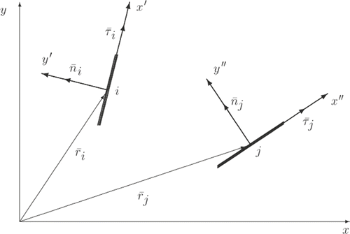
In order to formulate the linear algebraic system generated by the BEM, let us consider the arbitrary pair of elementary displacement discontinuities which are described, respectively, by the data and in the Cartesian coordinate system (x, y). Here the first two quantities designate coordinates of the central point, while vectors are directed along the elementary crack and in the direction of its normal (Figure 3). Let us study the contribution of j-th element to the normal and tangential stresses on i-th element. For this aim we couple the i-th and j-th cracks to the local Cartesian coordinate systems, (x′, y′) and (x′′, y′′), respectively. It is obvious from Figure 3 that if we denote by the radius vector of point i in the coordinate system (x′′, y′′) then (44) Therefore, in the coordinate system (x′′, y′′) we have (Equation (3.7)) (45) (46) (47) where quantities (x′′, y′′) = in the original coordinate system are given by (3.10).

Figure 3. Mutual influence of i-th and j-th elementary cracks.

If we still remain in the coordinate system (x′′, y′′) then in this system the normal and tangential stresses on the elementary i-th area can be calculated by using again Equations (3.8): (48) with quantities determined by (3.11).

We thus have finally derived a closed form for the influence of the displacement discontinuities , defined over a small elementary linear crack located at j-th node point with coordinates (x_j, y_j), unit normal and unit tangent , to the normal and tangential stresses, , acting over the faces of i-th elementary crack located at i-th node point (x_i, y_i), with unit normal and unit tangent . The sought expression is defined by Equation (3.12), where all quantities are defined in the basic coordinate system by Equations (3.10) and (3.11).

If the total number of elementary cracks is N then, due to linearity of the problem, the complete contribution of all elementary cracks to is a superposition of elementary expressions (3.12) that can be written symbolically as (49) for all elements i = 1, …, N. These relations contain 2N unknown quantities . Obviously, by using boundary conditions (3.4) applied for i-th crack, one can obtain the closed-form 2N × 2N linear algebraic system regarding these unknown quantities (50) with quantities , , being defined by expressions (3.3).

Let us assume that the US sensor is placed in a far zone to register longitudinal far-field wave signals scattered by the considered crack whose location and geometry are a priori unknown. Typically, recording longitudinal waves by an US transducer is equivalent to registration of the radial component of the displacement vector. In frames of very standard ‘echo-method’ the far-field pressure is measured just in the same direction α from which the incident wave arrives. It is obvious that if j-th elementary crack (x_j, y_j) is again defined by its unit normal and tangential vectors, , , then (51) where i_x and i_y are unit direction coordinate vectors in the basic coordinate system, and quantities are defined by formulae (2.14), with (x′′, y′′) substituted for (x, y).

The following asymptotic representations for a large argument are helpful to treat the far-field scattering (a certain inessential factor is omitted all over below): (52) (53) It is obvious that we have kept only longitudinal scattered component in Equations (3.16) and (3.17). It should also be noted that, due to (3.10), (54) that can be verified directly. Evidently, in the far zone, as R → ∞: (55)

Now, by combining expressions (3.15), (2.14), (3.16) with the following estimates valid for : (56) one can easily obtain the far-field scattering pattern, which is registered by a sensor of longitudinal waves, in the following way, written in the discrete form as a superposition of elementary contributions (3.15): (57)

4. Formulation of the reconstruction problem

If the crack geometry would be known then, after having numerically solved the basic system (3.14), one can define the quantities . Then one can calculate the far-field scattering diagram A(α) on the basis of Equation (3.19). This procedure is to solve the direct diffraction problem with the elastic waves process. The inverse reconstruction problem is to determine the contour ℓ defining crack's configuration, by knowing the input data on the registered scattered pattern A(α), 0 ≤ α ≤ 2π, for a fixed frequency. For such a reconstruction problem function A(α) is known; however, both crack's contour ℓ (i.e. quantities τ_jx, τ_jy, n_jx, n_jy) and quantities are unknown. If one describes contour ℓ by a certain parametric equations, then the full set of unknown functions consists of this new equation of the boundary plus a set of quantities over this contour.

It should be noted that the problem under consideration is ill-posed in the sense of Tikhonov 14, because the operator of the direct problem G : ℓ → A(α) is compact in any functional space naturally associated with the problem. Besides, the problem is nonlinear. These specific properties significantly complicate the numerical treatment of the reconstruction problem under consideration.

Let us approximate the boundary line of the flaw in the Cartesian coordinate system by the following parametric equations: (58) With such a treatment the basic unknown quantities are {a_m, b_m, c_m, d_m}, m = 1, …, M and their total number is 4M. Note that we omit the zeroth coefficients a₀, c₀ here since they are connected with the choice of Cartesian origin only.

If all these quantities are known then the boundary contour is known too, and one can numerically solve the basic system of boundary equations (3.14) written in the symbolic form: (59) Here is the unknown vector in linear algebraic system (4.2), while the right-hand side is determined by the incident wave. Matrix A is of dimension 2N × 2N.

The solution to linear algebraic system (4.2) can be expressed in terms of the inverse matrix, as follows: (60) Obviously, matrices A₁ and A₂, both of dimension N × 2N, depend upon all 4M parameters a_m, b_m, c_m, d_m, m = 1, …, M: A₁ = A₁(a_m, b_m, c_m, d_m), A₂ = A₂(a_m, b_m, c_m, d_m).

If cracks's contour ℓ is approximated by expressions (4.1) then system (2.1) is in fact defined over the interval 0 ≤ ζ ≤ π. In the discretization process the simplest way is to choose a dense set of nodes ζ_j to be uniformly distributed over the interval [0, π].

For the inverse reconstruction problem, when the input data is the back-scattered pattern (3.19), the quantities should be substituted from (4.3) into (3.19). In order to attain a fully discrete form of governing equations, a finite number of ‘directions of illumination’ (i.e. directions of incidence) α = α_q, q = 1, …, Q, may be taken, to be more specific, with a constant step: α_q = (q − 1/2)h_α, h_α = 2π/Q, symmetrically with respect to both the coordinate axes. This yields the strongly nonlinear system of algebraic equations: (61)

The only arbitrary quantities on the left-hand side of (4.4) are 4M coefficients {a_m, b_m, c_m, d_m} in the parametric form (4.1) of contour ℓ. It should also be noted that all other quantities in (4.4) are expressed through coefficients {a_m, b_m, c_m, d_m}: (62)

If parameters {a_m, b_m, c_m, d_m} are known then one can arrange the grid nodes (x_j, y_j), j = 1, …, N over contour ℓ. For all that, the components of the unit normal and tangent are (63) written in a symmetric form.

It is interesting to compare the number of unknown parameters and the number of equations in (4.4). As indicated above, the first quantity is 4M. Obviously, the second one is equal to the number of sensor positions, quantity Q. Subject to which quantity is greater among these two, system (4.4) may be underdetermined, overdetermined or well-determined. Obviously, the number of the sensor points may affect the precision of the reconstruction. However, the technique itself is universal with respect to this number. One can suppose the more sensor measurement points the higher the precision of the reconstruction. In order to provide a realistic reconstruction, the number of scanning angles, quantity Q must be greater than the number of the unknown parameters, quantity 4M.

The system of Equations (4.4) can be resolved by a minimization of the discrepancy functional: (64)

When providing the input data to solve the formulated reconstruction problem, in practice, the measurements on the back-scattered wave amplitude in any direction cannot be carried out with absolute precision. This predetermines the input data to be known with a certain error. Therefore, the proposed algorithm must guarantee the stability with respect to small perturbations of the input data. It should be noted that in the case of absolute precision in the input data the true geometry of the crack ℓ brings zero minimum value to functional Ω. However, the uniqueness in the inverse problem is out of the present study since we cannot prove that only true geometry of the crack makes the value of this functional trivial.

The minimization of functional (4.7) can be attained by any classical method of optimization 15,16. However, the main restriction of regular iterative schemes is that they give a local minimum of respective functional only. For this reason, in our numerical experiments we used a version of the method of global random search contiguous to the one described in detail in 17. This algorithm is developed to seek maxima, but it can be applied to minima too. It is so constructed that it moves both up and downhill and as the optimization process proceeds, it focuses on the most promising area. As a first step, it randomly chooses a trial point within the step of the user selected starting point. The function is evaluated at this trial point and its value is compared to its value at the initial point. In a maximization problem, all uphill moves are accepted and the algorithm continues from that trial point. Downhill moves may be accepted. It uses objective function F and the size of the downhill move in a probabilistic manner. The smaller F and the size of the downhill move are, the more likely that move will be accepted. The relationship between the initial value of F and the resulting step length is function dependent. This algorithm shows perfect convergence for many problems, also for our inverse problem, but unfortunately sometimes it arrives at a local extremum, instead of the global one, in the cases when there are a lot of global minima of the objective function.

The algorithm applied is a slight modification of this idea. It possesses the two following specific features: (1) random sampling of values in the neighbourhood of the points, for which the values of the functional are smaller, happens more frequently than in the neighbourhood of worse points and (2) the domains, in which random values of variables are chosen, are gradually contracted to the small neighbourhoods of the points with smaller values of the functional. This technique demonstrates remarkable convergence for all considered examples.

5. Some examples of reconstruction

To be more specific, let us test the proposed algorithm on the example of cracks whose boundary line is symmetric with respect to horizontal axis, and with M = 4 coefficients in approximation (3.1). We thus put all b_m, c_m = 0, m = 1, …, 4, so that the number of remaining unknown parameters a_m, d_m, m = 1, …, 4, here is 2M = 8.

In our numerical simulation we always put the longitudinal wave length to be two times longer than the transverse one: λ_p/λ_s = k_s/k_p = 2. For all examples listed below the input data for the reconstruction is taken from the solution of respective direct problem, with some stochastic perturbations of so obtained data, in order to model the input data with a certain error.

Let us estimate the efficiency of the proposed algorithm. All examples considered below are applied with 500 iterations in the described stochastic search, with 30 trials on each iteration step. The algorithm thus uses 30 × 500 = 15,000 trials of the objective functional Ω that takes near 10 min of calculations when implemented on PC with AMD Athlon Core2 processor of 6.0 HGz CPU clock (recall that each trial requires solution of the basic BIE system). If anyone would apply direct search by an enumerative technique, then one would calculate functional Ω depending upon desired scale in the precision of all 2M = 8 coefficients. In the poorest case one takes 10 values for each of these eight parameters a_m, d_m. Then in total, one should apply 10⁸ trials, that is by four orders greater than analogous quantity in the algorithm proposed here. It is obvious also that the calculation time for such ‘direct’ numerical experiments exceeds the capabilities of any existing computer.

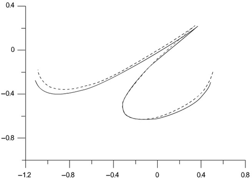
Some examples of the reconstruction are demonstrated in Figures 4–6, where all units of dimension of length are related to the longitudinal wave-length λ_p. As follows from the presented examples of reconstruction, precision of the input data is less significant for precision of the reconstruction. Typically, simpler geometries possess better reconstruction. However, the figures demonstrated show that complex geometries can be reconstructed by the proposed method with an admissible precision.

Figure 4. Reconstruction of a semi-circle crack, exact input data: solid line – true boundary contour; dashed line – reconstructed boundary.

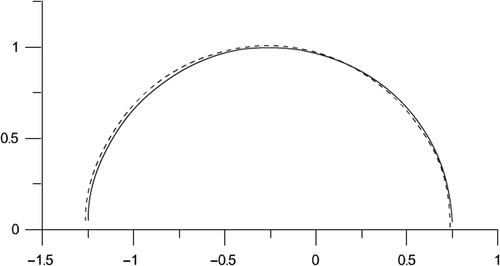
Figure 5. Reconstruction of a self-intersecting crack, 5% relative error in the input data: solid line – true boundary contour; dashed line – reconstructed boundary.

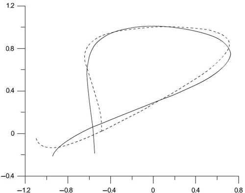
Figure 6. Reconstruction of a complex-shaped crack, 10% relative error in the input data: solid line – true boundary contour; dashed line – reconstructed boundary.

Acknowledgements

The present work has been supported in part by Italian Ministry of University. The work is also supported by Russian Federal Targeted Programme ‘Scientific and Scientific-Educational Personnel of Innovative Russia’ for 2009–2013, Project 02.740.11.5024.

References

- Krautkrämer, J, and Krautkrämer, H, 1983. Ultrasonic Testing of Materials. Berlin: Springer-Verlag; 1983.
- Colton, D, and Kress, R, 1983. Integral Equation Methods in Scattering Theory. New York: John Wiley & Sons; 1983.
- Colton, D, and Kress, R, 1992. Inverse Acoustic and Electromagnetic Scattering Theory. Berlin: Springer-Verlag; 1992.
- Potthast, R, 2001. Point Sources and Multipoles in Inverse Scattering Theory. London: Chapman & Hall; 2001.
- Friedman, A, and Vogelius, M, 1989. Determining cracks by boundary measurements, Indiana Univ. Math. J. 38 (1989), pp. 527–556.
- Andrieux, S, and Abda, AB, 1996. Identification of planar cracks by complete overdetermined data: Inversion formulae, Inverse Probl. 12 (1996), pp. 553–563.
- Bannour, T, Abda, AB, and Jaoua, M, 1997. A semi-explicit algorithm for the reconstruction of 3D planar cracks, Inverse Probl. 13 (1997), pp. 899–917.
- Abda, AB, Kallel, M, Leblond, J, and Marmorat, J-P, 2002. Line segment crack recovery from incomplete boundary data, Inverse Probl. 18 (2002), pp. 1057–1077.
- Alessandrini, G, Beretta, E, and Vessella, S, 1996. Determining linear cracks by boundary measurements: Lipschitz stability, SIAM J. Math. Anal. 27 (1996), pp. 361–375.
- Crouch, SL, and Starfield, AM, 1983. Boundary Element Methods in Solid Mechanics. London: George Allen & Unwin; 1983.
- Yin, HP, and Ehrlacher, A, 1993. Variational approach of displacement discontinuity method and application to crack problems, Int. J. Fract. 63 (1993), pp. 135–153.
- Li, H, Liu, CL, Mizuta, Y, and Kayupov, MA, 2001. Crack edge element of three-dimensional displacement discontinuity method with boundary division into triangular leaf elements, Commun. Numer. Methods Eng. 17 (2001), pp. 365–378.
- Abramowitz, M, and Stegun, IA, 1968. Handbook of Mathematical Functions, . New York: Dover; 1968.
- Tikhonov, AN, and Arsenin, VY, 1977. Solutions of Ill-posed Problems. Washington, DC: Winston; 1977.
- Kantorovich, LV, and Akilov, GP, 1982. Functional Analysis. Oxford: Pergamon Press; 1982.
- Gill, PE, Murray, W, and Wright, MH, 1981. Practical Optimization. London: Academic Press; 1981.
- Corana, M, Marchesi, M, Martini, C, and Ridella, S, 1987. Minimizing multimodal functions of continuous variables with the simulated annealing algorithm, ACM Trans. Math. Software 13 (1987), pp. 262–280.