Optimal modified method for a fractional-diffusion inverse heat conduction problem

Abstract

We consider the determination of the boundary temperature from one measured transient data temperature at some interior point of a one-dimensional semi-infinite conductor. Mathematically, it can be formulated as a fractional-diffusion inverse heat conduction problem where data are given at x = l and we want to determine a solution for 0 < x < l. This problem arises in several contexts and has important applications in science and engineering. The difficulty of the problem is its severe ill-posedness, i.e. the solution (if it exists) does not depend continuously on the data. In this article, we consider an optimal modified method from the frequency domain and obtain a Hölder-type convergence estimate with the coefficient c = 1, which is optimal. The method can be implemented numerically using discrete Fourier transforms. Three kinds of examples illustrate the behaviour of the proposed method.

Keywords:

• inverse problem
• ill-posed problem
• fractional inverse heat conduction problem
• regularization
• optimal estimate

1. Introduction

It is shown in 1–3 that the classical diffusion equation, requiring second spatial derivatives and first time derivatives can be reduced to a simpler equation involving only a first-order spatial derivative and a half-order time derivative under the assumptions of linear unidirectional heat transport through a semi-infinite domain with common constant initial and asymptotic boundary conditions.

The fractional partial derivative equation is then utilized to recover the temperature at the active boundary from the knowledge of the analytic temperature function given also at the active boundary. Some recent discussions on diffusion processes involving fractional derivative formulations for direct problems (superdiffusion, non-Gaussian diffusion) can be found, for example, in 4,5 and the references therein.

In this article we study the more general ill-posed problem of attempting to recover the temperature function at the active boundary from one measurement of the transient temperature function at some arbitrary interior space location of the semi-infinite domain. Mathematically, the data are given at x = l and we want to determine a solution for 0 < x < l. The difficulty of the problem is that the solution (if it exists) does not depend continuously on the data. Murio 1,6 studied the problem using his mollification method, and obtained some nice numerical results. Our main aim is to present and analyse a regularization method, based on a modification of the exact ‘kernel’ in the frequency domain, for stable numerical computation of the boundary functions. We give and prove a Hölder-type convergence estimate with the coefficient c = 1 which shows that the proposed method is an optimal regularization method, in the sense of Tautenhahn 7. Three kinds of interesting examples are given to illustrate the computed behaviour of the proposed method.

In what follows we refer to this problem as the fractional inverse heat conduction problem (FIHCP). It should be noticed that Beck et al. in 8 and Alifanov et al. in 9 discussed various numerical approaches for the usual inverse heat conduction problem (IHCP) which requires second spatial derivative and first time derivative, while this article considered a factional IHCP which only requires a first-order spatial derivative and a half-order time derivative. We are mainly devoted to the optimal convergence estimates in the sense of Tautenhahn 7.

The half-fractional time derivative that appears in the FIHCP corresponds to the Riemann–Liouville definition.

The Riemann–Liouville fractional derivative of order α, 0 < α < 1, of an integrable function g defined on the interval [0, T], is given by the convolution integral where Γ(·) is the Gamma function.

2. Ill-posedness of problem and regularization

We consider a one-dimensional FIHCP in a quarter plane (x > 0, t > 0) in which the temperature f(t) = u(0, t) on the active boundary (x = 0) is desired and unknown, and the temperature g(t) at some interior point x = l(l > 0) is approximately measurable. We assume a normalized (dimensionless) linear heat conduction with constant diffusivity and common constant initial temperature distribution and asymptotic boundary temperature. Following 1,6, the mathematical description of the FIHCP is listed next. The unknown temperature u(x, t) satisfies (1) where a is the constant diffusivity coefficient, u_∞ = u(x, 0) = lim_x→∞u(x, t) = const, and the half-time differentiation indicates the Riemann–Liouville fractional derivative.

In 1,6, Murio mainly considered the numerical computation of the FIHCP and gives few theory results. Our goal in this article is to gives the optimal convergence estimates for the FIHCP. We also use some numerical results to show that the considered method can be implemented and is effective.

For some linear ill-posed problems, we can get the explicit expression of solution in the frequency domain by using the Fourier transform techniques. Consequently one could clearly know the ill-posedness of the discussed problem and conveniently prove some stability and convergence results. Actually, the Fourier transform technique has been extensively used, please refer to 10,11 and references therein.

In order to using the Fourier transform techniques of the FIHCP, and in the rest of the article, we assume without loss of generality, a = 1, u_∞ = 0 and all the functions extended to the whole line −∞ < t < ∞ by defining them to be zero for t < 0 whenever it is necessary. We also assume that all the functions with respect to the time variable t are in L²(ℝ) and use the corresponding L² norm.

2.1. Analysis of ill-posedness

We define the Fourier transform of g(t) as (2) In working with the Fourier transform we will consistently use s for the transform variable, and for transforms of functions we will use the corresponding capital letters, e.g. F = ℱf.

Fourier transforming (1) with respect to time variable t, we can formulate the solution u, in the frequency space, as (3) where denotes the principal value of the square root,

Since the real part of is positive and our solution U(x, s) with respect to s is assumed to be in L²(ℝ), we see that, for 0 < x < l the exact data function, G(s), must decay rapidly as |s| → ∞. However the data g in problem (1) are generally based on (physical) observations and we only have the noisy data g^δ ∈ L²(ℝ)) with ‖g − g^δ‖_L²(ℝ) ≤ δ. Since we cannot expect the measurement data G^δ(s) have the same decay in frequency domain as the exact data G(s), the solution will not, in general, be in L²(ℝ) for fixed 0 ≤ x < l. Thus, if we try to solve the problem (1) numerically, high-frequency components in the error, δ, are magnified and can destroy the solution.

In the following, we are interested in the solution in the interval 0 < x < l. Usually, for a stable numerical approximation of the solution u of problem (1) some regularization technique has to be applied, which provides a sequence of approximations with as δ → 0 under proper choice of the regularization parameter α, where R_α is a regularization operator (usually bounded). Hence, regularized solution depends continuously on the data. However, as is typical for ill-posed problems, the convergence of to u can be arbitrarily slow if we do not impose additional a priori restrictions on the unknown solution u. Quantitative a priori restrictions that will work in different ill-posed problems (and enable us to overcome the ill-posedness) consist in imposing a bound E on the (unknown) solution.

Let us restrict our quantitative a priori information concerning u as (4) where E > 0 is a constant.

2.2. Regularization

The analysis of above subsection tell us that the real cause of ill-posedness is the noise of data in the high-frequency components blows up the solution. That is the noise in the measurement data G^δ will be infinitely amplified by the impact . Thus, from formula (3), we have two ways to solve the concrete inverse problems. One way is to eliminate the noise in the high-frequency components through mollifying the noisy data 1,6. The other way is to eliminate the high-frequency effect through modifying the ‘kernel’ . In this article we shall study the latter.

For the convenience of discussing, we rewrite the formula (3) as (5) where

Motivated by the references 11–13, we discuss a regularization method for the fractional-diffusion IHCP (1) in the frequency domain through modifying the exact ‘kernel’ e^{(l−x)(a+bi)}, i.e. according to (6) or equivalently (7) where the modified ‘kernel’ satisfies The choice of β, which plays the role of regularization parameter, is based on some a priori knowledge about the magnitude of the errors in the data g.

3. Convergence estimate

Before analysing the properties of the modified ‘kernel’ κ_β(x, s) in the formula (6) three points are highlighted: (a) the modulus of the modified kernel is less than or equal to the modulus of the exact kernel, i.e. |κ_β(x, s)| ≤ |e^{(l−x)(a+bi)}|; (b) the κ_β(x, s) completely reserves the low-frequency components (i.e. for small |s|, the constructed new ‘kernel’ equals the exact ‘kernel’ = e^{(l−x)(a+bi)}), since these components contain the main information of solution; (c) the κ_β(x, s) eliminates the effect of high-frequency components (i.e. the new ‘kernel’ is bounded even if |s| tends to infinity), since these components are the natural cause of producing ill-posedness. The property (b) guarantees that the constructed regularization solution is an approximation of the exact one. Obviously, the larger the parameter β, the better the degree. Property (c) describes the degree of continuous dependence, i.e. when the κ_β(x, s) is bounded, the regularized solution will depend continuously on the data. Furthermore, the smaller the parameter β, the better the degree of the regularized solution depends continuously on the data. Consequently, we need a strategy to choose the parameter β in order to keep the balance between the properties (b) and (c).

In the following, we shall give our main results.

THEOREM 3.1

If the measured data g^δ satisfy ‖g − g^δ‖ ≤ δ, then

i.	The regularization solution (6) is continuously dependent on the data.
ii.	Let u be the solution of problem (1) and let be the regularized solution. Assume that the a priori bound (4) holds. Then, for fixed 0 < x < 1, Furthermore, if the regularization parameter β is chosen optimally by (8) there holds the optimal estimate for fixed 0 < x < l, (9)

We transfer the proofs of Theorems 3.1 and 3.2 to the appendix, since (i) our main aim is to present the optimal convergence results, (ii) one can apply Theorem 6.2 of reference 7 to prove our Theorem 3.1 and (iii) one can refer to a similar process of the proof 14 in which Qian gives an optimal result for a two-dimensional IHCP.

Actually, our problem can be divided into both cases 0 < x < l and x = 0. For the former, the a priori bound ‖u(0, ·)‖ is sufficient. However for the latter, the stronger a priori bound ‖u(0, ·)‖_p (p > 0, defining in the formula (9)) must be introduced (cf. 11, Remark 3.2]). The corresponding choice of parameter β is also different. Thus, Theorem 3.1 gives an optimal convergence estimate for 0 < x < l; however, it is invalid at the end-point x = 0. This is common in the theory of ill-posed problems, if we do not have additional conditions on the smoothness of the solution at this boundary. To retain the convergence of the solution at x = 0, we shall introduce a stronger a priori assumption than (4). (10) where ‖ · ‖_p denotes the norm in Sobolev space H^p(ℝ) defined by

THEOREM 3.2

Let u be the solution of problem (1) with the exact data and let be the regularized solution given by (6) where the parameter β is chosen as (11) then there holds the convergence estimate, (12)

Both Theorems 3.1 and 3.2 show the optimal convergent rate for the fractional-diffusion IHCP (1) in the sense of Tautenhahn 7,13.

4. Numerical implementation

A numerical procedure for the optimal modified method can be based on the discrete Fourier transform (DFT). Out of necessity the data function g^δ must be sampled over a finite interval, which, without loss of generality, we can assume to be [0, 1]. The data function is sampled equidistantly. In using the DFT, it is assumed that the sequence to be transformed is periodic. In our application it is not natural to presuppose that the data vectors are periodic. Thus we shall make the data vector periodic before computation (please refer to 9, Appendix] for the process of periodization).

To illustrate the behaviour of the optimal modified method we constructed the test problems with a given function f, sampled at N = 101 equidistant points over [0, 1]. Then we computed a data function g at x = 1 according to which is well-posed. We usually think that the computed data g is exact. To this function we add a random perturbation and get the noisy data g^δ, i.e. (13) where (14) (15) The function ‘randn(·)’ generates arrays of random numbers whose elements are normally distributed with mean 0, variance σ² = 1 and standard deviation σ = 1. ‘randn(size(g))’ returns an array of random entries which is the same size as g. Finally, we use the optimal modified method (according to formula (6)) to obtain the numerical solution.

Example 4.1

Consider a smooth function

Figure 1(a) shows the exact and noisy data at x = 1, where we add the noise ϵ = 0.02 (about 3% level of noise in the experimental data) according to (12). Figure 1(b) shows that if directly using the formula (3) with noisy data, i.e. no regularization, we find that the computed solution blows up, which shows the reason why we need to employ the regularization method.

Figure 2(a)–(d) shows the regularized solutions at different locations, x = 0, 0.1, 0.5, 0.9. From formula (3) we know that the ill-posedness of problem (1) becomes worse and worse if the location x is farther from the measure location x = l. Figure 2(a) shows that the computed result is not very well at x = 0 which is farthest from the location x = l. However, the better the result, the closer the computed point is to the measure location, e.g. the result is quite satisfactory at x = 0.9 (Figure 2(d)).

In order to test the sensitivity of the method, i.e. the regularization role of the parameter β, we give Figure 3 in which we consider the location x = 0.5, the error ϵ = 0.02 (see formula (12), about 3%). The results from Figure 3 indicate that the quality of the numerical solution is not very sensitive to variations of the parameter β. It is the author's experience that, in practice, it is relatively easy to find an appropriate value for β.

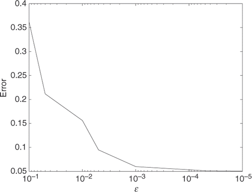
We also made a series of experiments with smaller and smaller perturbations of the data in order to study the behaviour of the error in the regularized solution as ϵ → 0. These computations are illustrated in Figure 4, which shows the nice convergence.

To further show the computed behaviour of the proposed method, we give two more examples, in which we are interested in the location x = 0, since the results of computation at other location (i.e. x > 0) are better than that at x = 0.

Figure 1. (a) Exact and noisy data at x = 1, the noise about 3% and (b) exact and unregularized solutions at x = 0.

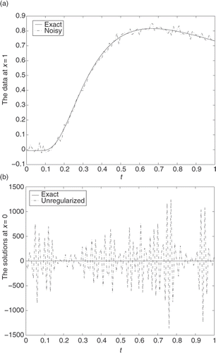
Figure 2. (a), (b), (c), (d) Correspond to the solutions at x = 0, 0.1, 0.5, 0.9, respectively.

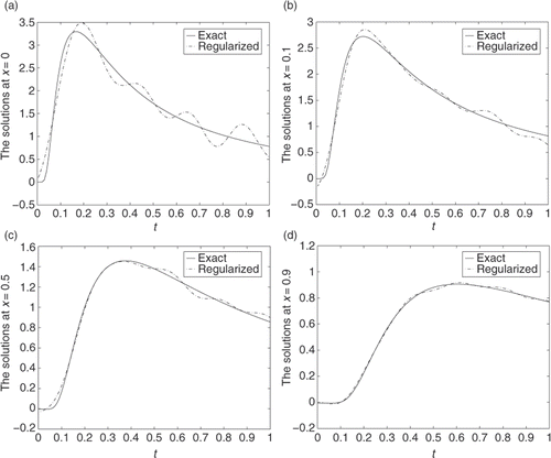
Figure 3. The error of l² norm vs. the 1/β at x = 0.5.

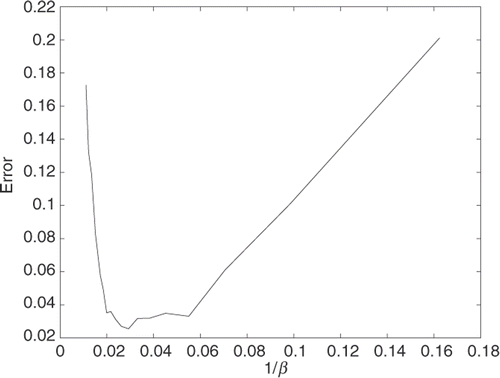
Figure 4. The error of l² norm vs. the noise ϵ at x = 0.

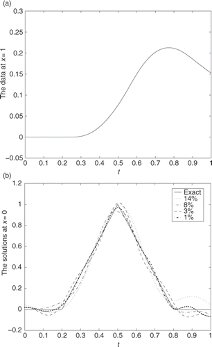
Example 4.2

Consider a continuous but not smooth function

Figure 5(a) shows the computed data g at x = 1. In Figure 5(b), we give the comparison of computing effect at x = 0 when adding different errors level to the data g. Through changing the value of ϵ in the formula (12), we add 14%, 8%, 3%, 1% levels of noise to the experimental data. These results show the better effect of computation.

Figure 5. (a) The computed data at x = 1 and (b) the regularized solutions at x = 0.

Example 4.3

Consider a discontinuous function

Figure 6(a) shows the computed data g at x = 1. In Figure 6(b), we give the comparison of computing effect at x = 0 when adding different errors level to the data g. Through changing the value of ϵ in the formula (12), we add 8%, 3%, 1% levels of noise to the experimental data. These results show the better effect of computation.

Figure 6. (a) The computed data at x = 1 and (b) the regularized solutions at x = 0.

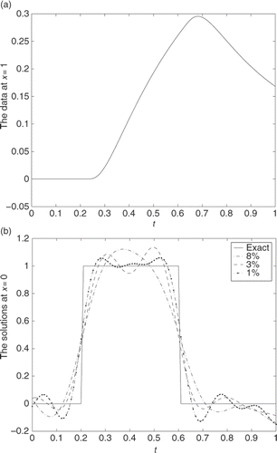
Remark 4.4

We choose Example 4.3 from Murio 1,6. The difference is that Murio considered the measurement data g^δ at x = 0.5, while we considered at x = 1. From formula (3) we know that the farther the computed location, the more severe the ill-posedness of problem (1). Consequently, our test is sharper. If we also consider the measurement data g^δ at x = 0.5, we have similar computing effect to that in Murio 1,6.

The numerical experiments indicate that the modified method works well for problems with small measurement errors. For problems with higher error levels, the results are less encouraging. However, the modified method can be combined with initial filtering of the data 1, which reduces the sensitivity to perturbations in the data. Such initial filtering can be easily used here. The main purpose of this article is to give the optimal convergence estimate for the FIHCP and use several examples to validate the effectiveness of the modified method.

Acknowledgements

The author wishes to thank the anonymous referees for their valuable comments and suggestions, which lead to the present improved version. The author also acknowledges the China Postdoctoral Science Foundation funded project (Nos. 20080440157, 200902511) and Jiangsu Planned Projects for Postdoctoral Research Funds (No. 0802004C).

Appendix

Since the regularization method (6) is constructed from the frequency domain, we could conveniently prove our results by using the Fourier transform techniques. The following process of proof confirms this fact.

Proof of Theorem 3.1

We first prove the continuity of the regularization solution (6). Without loss of generality, suppose that we have two regularized solutions u_β and defined by (6) with data g and g_δ which satisfies ‖g − g_δ‖ ≤ δ, using Parseval's equality, then (16) which proved the part (i) of Theorem 3.1.

We now prove the regularized solution u_β in formula (6) for how to approximate the exact solution u of problem (1) with the same exact data g. (17) Consequently, (18) Let . Differentiating h(a) and setting the derivative equal to zero, we find (19) Therefore, we have from (18) that (20) Now combining (15) and (20) with the triangle inequality, we have (21) Minimizing the function η(β), we find that (22) is the minimizer, i.e. . Consequently, inserting (22) in (21), we have which is just the estimate (8).▪

Proof of Theorem 3.2

Following the process of proof of Theorem 3.1, we have Let . Differentiating h(s) and setting the derivative equal to zero, we find Therefore, where we have also used the formula (10).▪

References

- Murio, DA, 2007. Stable numerical solution of a fractional-diffusion inverse heat conduction problem, Comput. Math. Appl. 53 (2007), pp. 1492–1501.
- Oldham, KB, and Spanier, J, 1970. The replacement of Fick's law by a formulation involving semidifferentiation, J. Electroanal. Chem. 26 (1970), pp. 331–341.
- Oldham, KB, and Spanier, J, 1972. A general solution of the diffusion equation for semiinfinite geometries, J. Math. Anal. Appl. 39 (1972), pp. 655–669.
- Liu, F, Anh, V, and Turner, I, 2004. Numerical solution of the space fractional Fokker-Planck equation, J. Comput. Appl. Math. 166 (2004), pp. 209–219.
- Meerschaert, MM, and Tadjeran, C, 2004. Finite difference approximations for fractional advection-dispersion flow equations, J. Comput. Appl. Math. 172 (2004), pp. 65–77.
- Murio, DA, 2009. Stable numerical evaluation of Grünwald–Letnikov fractional derivatives applied to a fractional IHCP, Inverse Probl. Sci Eng. 17 (2009), pp. 229–243.
- Tautenhahn, U, 1998. Optimality for ill-posed problems under general source conditions, Numer. Funct. Anal. Optim. 19 (1998), pp. 377–398.
- Beck, JV, Blackwell, B, and Clair, SR, 1985. Inverse Heat Conduction: Ill-posed Problems. New York: Wiley; 1985.
- Alifanov, OM, Artioukhine, EA, and Rumyantsev, SV, 1995. Extreme Methods for Solving Ill-Posed Problems with Applications to Inverse Heat Transfer Problems. New York: Begel House; 1995.
- Eldén, L, Berntsson, F, and Regińska, T, 2000. Wavelet and Fourier methods for solving the sideways heat equation, SIAM J. Sci. Comput. 21 (2000), pp. 2187–2205.
- Qian, Z, and Fu, CL, 2007. Regularization strategies for a two-dimensional inverse heat conduction problem, Inverse Probl. 23 (2007), pp. 1053–1068.
- Seidman, TI, and Eldén, L, 1990. An ‘optimal filtering’ method for the sideways heat equation, Inverse Probl. 6 (1990), pp. 681–696.
- Tautenhahn, U, 1997. Optimal stable approximations for the sideways heat equation, J. Inverse Ill-posed Probl. 5 (1997), pp. 287–307.
- Qian, Z, 2009. An optimal modified method for a two-dimensional inverse heat conduction problem, J. Math. Phys. 50 (2009), p. 023502, 1–9.