Estimation of parameters for dynamic volume spline models

Abstract

Soft tissue models are of many types, but each type has its own problems in terms of realistic appearance and computational efficiency. In this study, we propose a hybrid model based on dynamic volume splines which combine the advantages of these models. To simulate a realistic appearance, biomechanical properties of the real tissue are obtained by force–displacement experiments and used to tune the parameters of the model. Unlike the usual types described in the literature, a new experiment is proposed where displacement is measured not only for the point of force application but also for the region around the applied force. In our study, multiple camera views were used to enable 3D reconstruction of the surface. The differences arising between the surfaces obtained before and after the application of force were then used in optimization-based inverse solution methods, and the estimated parameters were found to be consistent with the biomechanical tissue properties described in the literature.

Keywords:

• dynamic soft tissue model
• 3D reconstruction
• surface fitting
• parameter estimation
• inverse solution
• optimization

1. Motivation and content

Various methods are proposed in the literature 1–5 for soft tissue modelling. The performance of these methods is evaluated according to the computational load they require and the extent of realism of appearance achieved in representing the real tissue. For example, FEM models need appreciable computation time, but results achieved are more realistic unlike the surface/volume models whose simulations are not so realistic but computation time is less. In this study, the hybrid type model we propose for facial soft tissue simulation is a dynamic volume spline-based model.

The performance of the proposed model needed to be tested against the real living tissue with setting at the most suitable optimum model parameter. The behaviour of the living tissue for both of these activities was observed by means of appropriate experiments and compared with the behaviour of a model under the same conditions. The technique most prevalent is to extract information from the tissues removed from a living organ. However, since the behaviour of tissue changes when it is removed from the organ, the estimated parameters derived in this manner usually do not represent those of the actual tissue. Therefore, experiments should be performed on living tissue (in vivo). Most experiments consist of applying force on the tissue and measuring the displacement only at the point of application of the force. However, this is grossly inadequate since the deformation of tissue is not only limited to the point of force application but also affects the deformed region around it, which could provide more information about behaviour of the tissue. In this study, we propose a force–displacement type of experiment where we measure the deformation not only at the point of force application but also for a region around the applied force. Using a multicamera system with macro lenses, we obtained detailed and high-resolution images and reconstructed the 3D shape of the surface before and after the application of force. In this manner, we observed the displacement on the tissue not only at the point of force application but also for the whole extent of the deformation. This yielded us more information than only at the point contact of force.

We used observed behaviour of the tissue from the experiment described above, applying its inverse solution techniques to obtain the model parameters for our proposed model. Applying optimization-based inverse solution techniques, we estimated the model parameters. We then observed that when these estimated parameters were used in our model, its behaviour resembled the real living tissue.

The purpose of this article is not only to discuss the success of the proposed model, but also to describe our experiment and the manner in which an inverse solution can be used to estimate the parameters of a volume spline model so that the model behaves realistically. The method is not only limited to the proposed type of model but also could be applied to various other models as well.

Section 2 is a survey of literature on experiments performed on tissue properties and model parameter estimation. In Section 3, we review the tissue parameter values contained in the literature. In Section 4, we explain the dynamic volume spline model of soft tissue. In Section 5, we describe our experiment. In Section 6, we explain the application of an inverse solution algorithm to estimate the model parameters for the proposed model described in Section 4 and its use as the forward solution. The information obtained from the experiment explained in Section 5 is used to construct and optimize the objective function. Finally, results are given in Section 7 with concluding remarks. Suggestions for future work are presented in Section 8.

2. Previous studies

There are two major problems in constructing realistic soft tissue simulators. One is the extraction of real biomechanical information from living tissue and the other is testing and verification of the model against the real tissue 6. Various experiments are performed on living tissue or after removing the tissue from the living body. In vitro experiments use the specimen extracted from the living organ 7, whereas in vivo experiments are directly performed on the living organ. However, when the tissue is taken out of the organ, its behaviour could change. But experimenting on the living tissue is highly complicated because the measurement devices should not cause any harm to the living body. Therefore, the equipment should be safe and ergonomic.

In nearly all of the living tissue experiments, behaviour is observed on a single axis. There are basically two types of experiments: aspiration-displacement 8 or loading-deformation 7. In 9, a mass spring model is proposed for a human thigh and the model parameters are obtained by measuring the applied forces and displacements on various parts of the living thigh. In 10, the behaviour of the thigh tissue through time is measured when a force is applied. In 11, various experiments such as stretch, draw, twist, and aspiration are performed on the forearm and forehead in order to extract information about properties of the skin. In 12, it is stated that the estimated parameters differ appreciably from experiment to experiment.

Lately, medical imaging is also used to estimate biomechanical tissue properties. For example, in 12, tissue is modelled using a very simple equation relating pressure and deformation. Aspiration is used for measuring skin thickness and elasticity, and ultrasound for the extent of stretching at the point of force. When modelling by FEM is used, a similar approach is adopted 13–15. In 15,16, a Hounsfield unit is used in facial CT imaging to estimate the resistance of facial skin against force. Magnetic resonance imaging (MRI) is used in 17 to measure the elasticity of brain tissue. In some other more precise experiments, resistance to elasticity is measured by the application of magnetic resonance elastography (MRE) 17.

3. Tissue properties in the literature

There are some studies in the literature that define the tissue properties for the skin-fat tissue layer that we are trying to model. However, these parameters differ for various regions on the facial area and also from person to person. In this section, we try to briefly describe the values given in the literature for the mass, damping, and elasticity properties of skin.

3.1. Mass

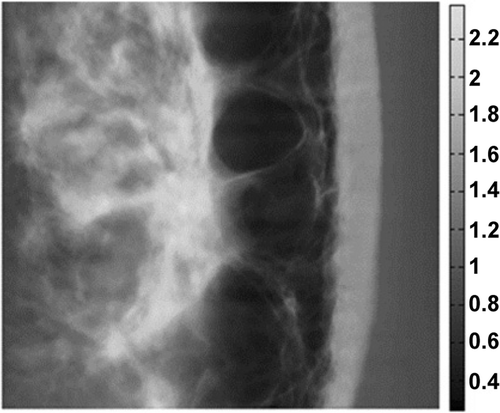
It is impossible to define the mass density for human skin as it is highly heterogeneous and anisotropic; that of the skin on the surface reveals some variations while the fat below has a lower density (Figure 1). In 18, various mass density values for different regions of a soft tissue are estimated using different medical imaging techniques such as diffraction enhanced imaging (DEI) and multiple image radiography (MIR). Based on 18, this study assumed the mass density for human facial skin as 0.0005 kg m³.

Figure 1. Estimation of soft tissue mass density for a woman’s breast in units of g cm⁻² 18.

3.2. Damping (friction)

Friction offers nonlinear properties for a material such as human tissue. Besides its heterogeneous behaviour, skin consists of holes filled with water and it is impossible to measure its damping value. To measure the damping coefficient, the hysteresis in the force–displacement graph of the human skin should be investigated. In other words, the damping coefficient of the skin could be estimated if the time required for a deformed skin to recover its original shape could be measured. Some values for the skin damping coefficient are also estimated during experiments performed to estimate skin elasticity 18.

In our model, we used a constant value for the damping coefficient and we set an appropriate value, which was decided heuristically. There are two reasons for this. One is that it is very difficult to obtain a damping coefficient from the skin and the fat layers. Even if it is measured, it is evident that the value will differ with different values of some variables such as temperature and skin density. The second reason is that the final steady state under an applied force in a second-order dynamical system such as ours will be independent of the damping coefficient. In other words, while the small displacement on facial skin is being computed, the difference in the damping coefficient will only affect the transient state, but will have no effect on the final steady state shape of the facial skin 19.

Since in our model we do not consider the transient response but consider the steady state response only, using an average damping value does not prevent us from estimating the subject specific elasticity value. Therefore, it was only important to use an appropriate damping value such that our system reached the steady state in the shortest time.

3.3. Elasticity

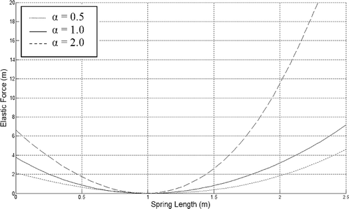
There are many studies in the literature that measure the elasticity value. In their experiments, the required force per unit extension is measured when the tissue is extracted from the organ. However, the skin loses its property of elasticity completely whenever it is separated from the living organ and the skin behaves as some other material. Generally, soft tissue is represented by nonlinear force–displacement graphics consistent with its inheterogeneous properties. Various functions are used to model this behaviour. For example, the following formula is used in 20 to model the behaviour represented in Figure 2: (1) In this nonlinear function, represents the absolute extension and d_ij represents the initial length between the two points, x_i and x_j. The proposed function for different k₀ values produces the figure shown. This function is used as the elasticity function in our model too. Here, elasticity is represented by the parameter α and as assumed to be 10 N mm⁻¹ 18.

Figure 2. Function given in (3) for various k₀ values.

4. Biomechanical model

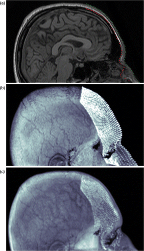
The soft tissue model possesses physical and anatomical properties of the skin such as thickness, viscoelasticity and mass density. The actual volume of the model is segmented from facial MR data. In this study, we developed a semi-automatic segmentation tool to extract the thin soft tissue volume of facial skin from the 3D MR data whose description follows. Two regular grids of size U × V are extracted from the outer and the inner surfaces of the soft tissue layer of the forehead (Figure 3). The outer surface is simply the face. The inner surface is the soft tissue boundary just above the fascia and the muscles. Since the grids are of the same size (U × V) and since points on the grids correspond to each other, the segmented volume is obtained as a grid of U × V × 2 points.

Figure 3. (Available in colour online). Semi-automatic localization of the the outer and inner surfaces of the thin soft tissue volume. Each surface is a uniform grid of U × V points. The volume constitutes a U × V × 2 grid. (a) Both layers (the outer (green line) and inner (red line) surfaces) visible are for a saggital slice. (b) The outer grid is depicted over the head, and (c) the inner grid is depicted over the head with transparency.

These U · V · 2 points are used to construct the volume spline, which is used to simulate the facial soft tissue. A volume spline of M × N × 2 grid of spline control points (where M ≤ U and N ≤ V) is fitted to cover all of the data points. The general volume spline equation can be written as (2) where V(u, v, w, B) is the 3D position of a point inside the volume in general coordinates (u, v, w), B_a,b,c's are the 3D control points of the volume spline and N.,. (.)'s, are the basis functions. Using the notation in 21, we may combine the basis functions in the Jacobian vector and represent (2) in matrix form as follows: (3) Here, B is matrix of size (M · N · 2) × 3, representing the control points in general coordinates: (4) J is a vector of size M · N · 2: (5) Then, by putting all the points in matrix notation, we may write (6) Here V is the matrix of data points (7) Finally, C is the matrix of Jacobian vectors for data points. C has the size of (U · V · 2) × (M · N · 2): (8) Assuming that U · V · 2 ≥ M · N · 2 and that the rank of C is maximal (equal to M · N · 2), the following equation will give us the control points covering the given volumetric data grid: (9) Using this formulation, the volume spline control points are fitted to the 3D data grid which is segmented from the MR data. However, for the model to possess physical properties, not only geometric properties but also the mechanical ones should be defined. The next subsection explains the dynamic behaviour of the volume spline model.

4.1. Dynamic volume spline model

Dynamic non-uniform rational B-splines (DNURBS) are introduced in 21 as a physics-based version of non-uniform rational B-splines (NURBS). DNURBS physics is established on the work–energy version of Lagrangian dynamics. The control points are considered as localized masses possessing localized stiffness and damping functions which are related to all parts of the surface via the Jacobian defined in (5). Consequently, the equation of motion is defined 21 as follows: (10) In this equation, T(t) is the total kinetic energy of the system, U(t) is the total elastic potential energy of the system, F_R(t) is Raleigh's dissipation energy, f(u, v, w) is the external force applied to the system and B(t) represents the control points in general coordinates as a function of time. We used precisely the same equation to identify the dynamics of motion for the control points of our model. Furthermore, we defined elastic and dissipation energies as stiffness and also damping matrices as defined in 21, except that in 21 these were defined for dynamic surfaces, whereas in our model we used volume splines. Thus, we had triple integrals for the three orthogonal parameter values u, v, and w, and defined the kinetic energy for our model as follows: (11) where μ(u, v, w) is the mass density function defined over the orthogonal (u, v, w) parameter space and is the time derivative of the points inside the spline volume. When we take derivatives on both sides of (5), we get the following equation: (12) Since the matrix J is obtained from the basis functions and is not a function of time, we define M by combining Equations (11) and (12) as follows: (13) where M is (14) Here M is a matrix of size (M · N · 2) × (M · N · 2), which represents localized masses for each control point and covariant relation of mass distribution among the control points.

Similarly, using the dissipation energy F_R(t), we obtained the (M · N · 2) × (M · N · 2) damping matrix D which represents the localized damping coefficients of the control points and the covariant relation of energy loss among them: (15) (16) Here, γ(u, v, w) is the damping density function defined over the (u, v, w) parameter space.

Qin and Terzpoulos 21 adopt the thin plate under tension energy model as the elastic potential energy model for DNURBS surfaces. Since this is a model intended for surfaces and as the thin plate is defined only for two dimensions, we had to modify the definition for three orthogonal dimensions as shown below: (17) Correspondingly, K is a matrix of size (M · N · 2) × (M · N · 2), which represents localized elastic relations among the control points and α(u, v, w) and β(u, v, w) are the elasticity functions which control local tension and rigidity, respectively. The matrix K is calculated as follows, where J_x is the first derivative of J with respect to x and J_xy is the second derivative with respect to x and y: (18) This matrix is the 3D version of the stiffness matrix defined in 21. Unlike in 21, here we updated it at each time-step of the dynamical equation according to the control point distances.

Finally, Equation (10) is rewritten in matrix form as follows: (19) where F_B(t) is the generalized force vector, obtained through the principle of virtual work done by the applied force distribution f(u, v, w): (20) Furthermore, I(t) is the moment of inertia which happens to be zero, since time derivative of J is zero. (21) Thus, we arrive at the final equation of motion as follows: (22) This can be rewritten as a system of differential equations: (23)

5. Experiment

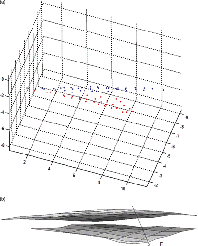
The experiment is based on the application of a very small force (0.17 or 0.25 N) on the skin and measuring the applied force and the deformation that occurs at and around the point of applied force (Figure 4). The force applied on the skin is measured with a force sensor of 0.01 N sensitivity and the deformed shapes of the skin before and after the application of force are viewed with multiple cameras (Figure 5). To make stereo matching easier, regular grid points are marked on the subject's face before commencing the experiment. Stereo analysis is performed between the image pairs, and the matched marks are extracted and the 3D locations of these points are reconstructed by triangulation (Figure 6a). Finally, spline surfaces 22 are fitted to these surfaces to enable the measurement of the differences between them (Figure 6b).

Figure 4. A very small force is applied to the subject’s forehead with a probe and the deformation viewed with multiple cameras.

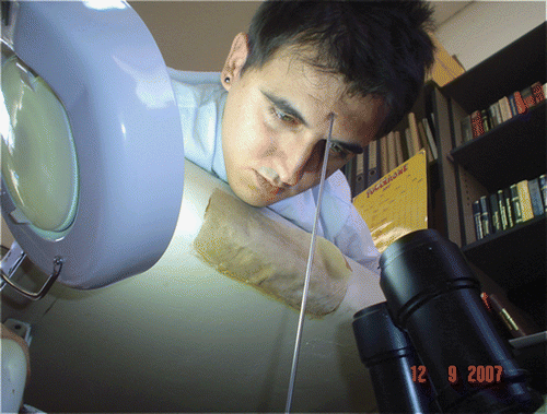
Figure 5. Stereo images recorded when force is not applied (top row) and when force is applied (bottom row).

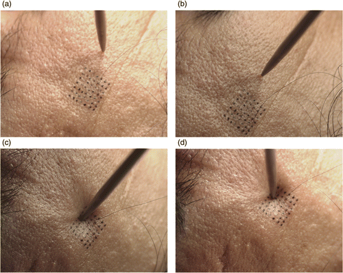
Figure 6. (Available in colour online). (a) 3D point cloud for the surface before the application of force (blue) and after the application of force (red) and (b) spline surfaces fitted to the point cloud surfaces. Yellow is the initial surface (before application of force) and red is the deformed surface (after application of force).

6. Parameter estimation by inverse solution

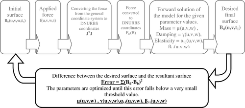
Our model is a volume spline model and the first step in modelling is to fit a volume spline to the shape to be modelled. The initial shape is the initial state of the model. Then, when a force is applied (F_B), this spline model is solved dynamically (23) based on its control points (B) using its parameters (M, K, D) until the model reaches a steady state, i.e. its new final shape. This is called the forward solution of the model. The inverse solution is applied to estimate the model parameters where the initial and the final shapes of the model are known. We estimate the parameters of our facial skin model using the inverse solution of the model where initial (before application of force) and final (after application of force) surfaces are obtained by the magnitude and the direction of the force applied during the experiment.

There is no closed form inverse solution for the model and some iterative optimization methods are needed. Details of the optimization system are given in Figure 7. Here, the indistinct coloured part is the forward solution. In the inverse solution, we initially obtain the forward solution of the model starting from the initial shape and using some preliminary values for the parameters. Then, the difference between the steady state forward solution and the desired solution, obtained from the experiment, is used as the objective function (24) and iteratively minimized with respect to the parameters.

Figure 7. Forward and inverse solution steps.

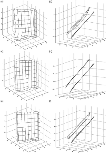
The objective function is computed as the sum of distances between corresponding control points on the surfaces: (24) where x is the parameter vector of our volume spline-based dynamic model and i is the index for the control points. The function forward (x) is the forward solution algorithm that uses predefined parameters, the initial surface and the applied force to calculate the final surface and bend is the deformed surface measured during the experiment when the same amount of force is applied on the surface of the face. In fact, the function f is the sum of squares formula, which is sometimes, for cosmetic reasons, multiplied by 1/2. Here, this function measures the Euclidean distances between the data obtained from our experimental measurements and those obtained from the model. This model is typically nonlinear in the unknown parameters. In other words, our function is the length of the corresponding residual (vector). For example, Figure 8(a) and (b) are different views of the face surface that is reconstructed during the experiment when a 0.17 N force is applied. This surface is used as bend. On the other hand, Figure 8(e, f) are different views of the surface computed by the forward solution of the model where a fictitious 0.17 N force is applied to the initial surface (Figure 8c, d). This surface is used as forward (x); bend and forward (x) are expected to come very close to each other when the model parameters are optimal. To minimize the squared difference (24), the ‘Nonlinear Least Squares (Gauss–Newton) method’, which is a simplified version of Newton's method, is used 23,24.

Figure 8. (a, b) Reconstructed 3D surface when 0.17 N is applied on the forehead, (c, d) initial surface used in the forward solution and (e, f) final surface formed by the forward solution of the model starting from the initial surface. All surfaces are shown from two different views by their spline control points.

6.1. Iterative optimization for the inverse solution

In Newton's method, the update equation for parameters of f in (24) is defined as follows: (25) where τ is used for iteration index, H is the Hessian matrix and ∇ is the gradient operator.

If we define and collect the differences at the control point pairs in a vector as follows: (26) sometimes (e.g. in nonlinear regression) also regarded as a row vector, then the gradient is defined as follows: (27) where J is the Jacobian matrix which is defined as (28) Because of the aforementioned nonlinearity in the parameters which are our decision variables, the Hessian of our function (needed when applying the iterative Newton's method for finding the ‘steps’) could hardly be computed. It is for reasons such as this that the so-called quasi-Newton methods have been developed in optimization theory. They aim at approximations of the Hessian (less expensive), rather than precisely quantifying it, and particularly, do not compute any second-order derivatives. Indeed, the quadratic character of our objective function gives rise to a very elegant ‘quadratic’ approximation of the Hessian by means of the objective function and its gradient (first-order derivatives). By this approximation, we arrive at the so-called Gauss–Newton method. In the Gauss–Newton method, the second derivative terms in the Hessian matrix are ignored assuming that near the solution for i = 1, …, N, and the Hessian is approximated by (29) so that the iteration (25) can be written in a simpler form as follows: (30) The drawback of this simplification (approximation) is that sometimes the convergence (to the real solution) is slowed down or does not take place by the Gauss–Newton method. For this reason, the so-called Levenberg–Marquardt method can be preferred for overcoming this drawback and regularizing the linear system for finding the ‘step’ by a well-controlled combination of both the Gauss–Newton and the ‘steepest-descent’ methods. This combination is also related with the so-called trust-region methods.

In fact, besides the Gauss–Newton method, many other nonlinear least-squares techniques can be interpreted as using an approximation of the second additive form in the formula for the Hessian, i.e. of (31) Levenberg–Marquardt's method uses the simplest of these approximation: (32) with some scalar . This approximation gives us the following linear system of the unknown step or increment vector q: (33) Often, one can find the Levenberg–Marquardt method implemented in the context of a trust-region algorithm. There, q may also be obtained by minimizing a quadratic model of the objective function with Gauss–Newton approximation of the Hessian: (34) Here, λ is indirectly determined by picking a value of Δ; the parameter Δ can be chosen based on the effectiveness of the Gauss–Newton method.

The Levenberg–Marquardt method may be understood as a mixture between the Gauss–Newton (if ) and the steepest-descent method (if λ is very large). An adaptive and sequential way of choosing λ and, by this, of the adjustment of mixture between the methods of Gauss–Newton and steepest-descent, is presented in 24. The term ‘ ‘can also be regarded as a regularization term that keeps the eigenvalues of away from 0.

6.2. Implementation

The optimization process was run on a desktop PC with an Intel Core 2 1.80 GHz processor and 1 GB memory using Linux operating system and Matlab R14 Optimization Toolbox. lsqnonlin (nonlinear least squares) was chosen as the optimization function. The usage of this function is as follows: where fun is the target function calculating B (control points) by calling the forward solution. It outputs the length of the resulting vector which is the difference between the expected B and the observed B.

x0	=	It contains the initial values of the unknown parameters. Since the purpose is to estimate the parameters μ, γ and α(u, v, w) of the forward solution, and x0 is the vector which is constituted by the initial values of those parameters.
lb	=	The constraint vector which is the lower bound of the parameters μ, γ and α(u, v, w).
ub	=	The constraint vector which is the upper bound of the parameters μ, γ and α(u, v, w).
x	=	The vector holding the values of the parameters found at the conclusion of the optimization process.

The surface obtained after the experiments were concluded was modelled as a 9 × 9 × 2 grid. Initial value for μ was taken as 0.0001 and α was initialized as 0.5 for all three directions (u, v and w). The damping coefficient, γ, used was 15. These values were selected from those stated in the literature and explained in Section 3.

The optimization was applied to two different data sets. One of the data sets were collected when a 0.17 N force was applied (Figure 8) and the other data when a 0.25 N force was applied (Figure 9). The resulting parameter values of each data set after the convergence are summarized in Table 1. Besides, the literature values are given in the last row of the table. For each data set, very similar shapes are computed which correlates the inverse solution and parameter estimation steps. Besides, the estimated parameter values are consistent with the values presented in the literature for human facial soft tissue.

Figure 9. Experimental data set 2: (a, b) surfaces reconstructed during the experiment when 0.25 Newton was applied on the face, (c, d) initial surface. Both surfaces are shown from two different viewing directions and (e, f) surface obtained when the model is solved when 0.25 N force was considered.

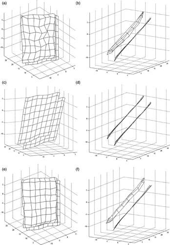
Table 1. Estimated model parameters for two experimental data sets and literature values (last row).

	μ (kg mm^−3)	αu (N mm^−1)	αv (N mm^−1)	αw (N mm^−1)
Experimental data set 1 (17 N)	0.0001	4.9999	0.2519	1.9135
Experimental data set 2 (25 N)	0.0017	2.6328	0.1830	1.7386
Literature values	0.0005	10	–	–

Remark In this study, we used refined methods of nonlinear regression, based on a model description, estimating and predicting our experimental data and of future states. In reality, sometimes a less detailed but practical model is preferred that benefits from very elementary basis functions which are much easier than, e.g. splines, but which at the same time allows the approximate representation of interactions between the input factors. Multivariate adaptive regression splines (MARS) is one such popular nonparametric regression and classification method, particularly useful for modelling nonlinear relationships that might exist among the variables 25. Recently, with our colleagues, we developed the CMARS (Continuous MARS) method 26–28 as an alternative to the backward stepwise part of the MARS. Our comparative studies indicate that CMARS performs better than MARS for modelling nonlinear relationships. In fact, it also turned out to be very competitive when used for the quality analysis in manufacturing or prediction of credit default in finance 26–29, and compared favourably with other data mining tools such as CART, neural networks and logistic regression. Since CMARS benefits greatly from the use of optimization techniques developed, namely, conic quadratic programming 30 with its efficient interior point methods 31, it suited our present study very well, and we intend to apply it in our future research studies.

7. Conclusion

In the literature, experiments of the force–displacement type are usually performed for only the point at which force is applied. However, in the experimental set up described in this study, the displacement can be computed for the neighbouring region of the applied force also by 3D reconstruction of multiple images. The critical step here is matching corresponding points between the stereo image pairs, and, in this study, this was done by marking a grid of points on the face. Automatic matching could also be done but such a grid of points also helps in recording the surfaces reconstructed before and after the application of force and also in superimposing the subject's face on the model.

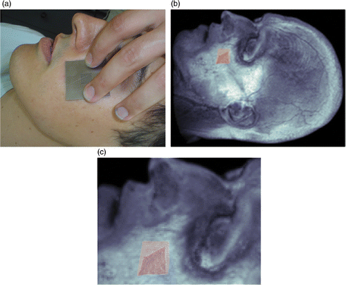
During the experiment, the reaction of the living tissue is measured when an external force is applied. When the same amount and type of virtual force is applied to the proposed tissue model, it should produce the same degree of deformation. Thus, the degree of similarity of the proposed tissue model to the real tissue is computed. The most critical step for achieving this is superimposing (registering) the experimental facial surface on the model. In Figure 10, the cheek part of the face is superimposed on the model.

Figure 10. Reconstructed surface is superimposed on the MR surface of the subject.

The main aim of the experiment was to obtain the model parameters that cause the model to behave like the facial soft tissue it replicates. The proposed model is a physical and mechanical model and its parameters correspond to the parameters of real tissue such as mass density and unit elasticity. Since the literature contains various values for these physical properties, we estimated them specifically to achieve better simulation quality of our model.

The other purpose of performing such an experiment was to assess the capability of our model in simulating real tissue. It is extremely difficult to model a complex material such as a human face which possesses anisotropic, heterogeneous, and nonlinear elasticity. As mentioned earlier in our literature survey, there is no model yet in terms of simulation quality and computation speed that can reproduce models of living tissue completely. Similarly, it is evident that our proposed model is not perfect. However, the tissue property values we obtained using the experimental data in this study are eminently consistent with the literature and encourage us to feel that our proposed model can be used in realistic soft tissue modelling.

Any skin specimen can be modelled with the volume spline. The dynamic behaviour of the specimen can be observed by the force–displacement experiment. Using the measured changes on the specimen in response to the applied force, the inverse solution can be applied and the parameters of the model estimated so that the model's behaviour resembles that of the actual specimen. This procedure can be applied to any region of the skin. But skin properties vary among people and among body regions. Thus, the experiment and the inverse solution should be applied to the region of the body that is to be modelled.

In the literature, the parameter value appearing for mass density is 0.0005 kg mm⁻³ and for elasticity on a single axis is 10.0 N mm⁻¹. The estimated parameter values for the experimental data set 1 was 0.0001 kg mm⁻³ for mass density and 4.9999, 0.2519 and 1.9135 N mm⁻¹ for elasticity on all of the three axes. The estimated parameter values for experimental data set 2 were 0.0017 kg mm⁻³ for mass density and 2.6328, 0.1830 and 1.7386 N mm⁻¹ for elasticity. Although the estimated values are highly consistent with the literature values in the order of magnitude, there are some differences. Some possible reasons can be listed as follows:

1.	Experimental steps such as positioning the subject, drawing the grid on the subject's face, imaging, measuring the force applied and reconstruction require accuracy of the highest order. Therefore, these steps have to be improved and can be achieved by using superior devices such as cameras and force sensors.
2.	Properties vary from person to person and hence are person-specific. These parameter values change even for the same person with changing age and health conditions. Thus, differences among the literature values are acceptable.
3.	Soft tissue parameter values also differ from region to region. Parameters for the thigh, head, face, and breast all differ from one another. Likewise, parameter values for breast soft tissue differ from those for facial skin.
4.	Furthermore, the literature gives parameter values for a single dimension. Although the experiments were conducted to ascertain the skin volumes, due to limitations in the measurements, the elasticity values were estimated using mostly single-dimensional models. Consequently, the parameter value for a single dimension was estimated. However, in our model, we used different elasticity values for the various dimensions (αu, αv, αw) and estimated all these parameter values. The elasticities in all these dimensions have a combined effect depending on the model volume and structure.

Notwithstanding all these differences, our results are consistent in the order of magnitude with those appearing in the literature. One important issue needs emphasis: the critical factor actually is not the consistency of the estimated parameters with the actual tissue parameters but the consistency of the model's behaviour with the behaviour of actual tissue when the estimated model parameters are applied to the model. On conclusion of inverse solution, the model parameters are determined so that the difference between the actual tissue shape and the model shape becomes negligible after the application of the real force and the simulated force, respectively.

A variance between the estimated values is usually encountered in complex experiments such as estimation of heterogeneous material properties. For this reason, experiments are usually replicated and the results are averaged to overcome this variance. We plan to perform more experiments and more inverse solutions (both on some simulated data and the real data) in a future study enable computation of the average.

Acknowledgements

This study is partially supported by TUBITAK 105E128 and BAP-2008-03-01-04.

References

- Sedef, M, Samur, E, and Başdoğan, Ç, 2006. Real-time finite-element simulation of linear viscoelastic tissue behavior based on experimental data, IEEE Comput. Graphics Appl. 26 (2006), pp. 58–68.
- Debunne, G, Desbrun, M, Cani, MP, and Barr, AH, 2001. "Dynamic real-time deformations using space & time adaptive sampling". In: Proceedings of Siggraph. Los Angeles, CA: ACM Press; 2001. pp. 31–36.
- Hauth, M, Groß, J, and Straßer, W, 2003. "Interactive physically based solid dynamics". In: Proceedings of the Eurographics/Siggraph Symposium of Computer Animation. San Diego, CA: Eurographics Association; 2003. pp. 17–27.
- Schoner, JL, Lang, J, and Seidel, HP, 2004. Measurement-based interactive simulation of viscoelastic solids, Comput. Graphics Forum 23 (2004), pp. 547–556.
- Schwartz, JM, Denninger, M, Rancourt, D, Moisan, C, and Laurendeau, D, 2005. Modeling liver tissue properties using a non-linear visco-elastic model for surgery simulation, Med. Image Anal. 9 (2005), pp. 103–112.
- H. Delingette, Towards realistic soft tissue modeling in medical simulation, INRIA. Report No. 3506. September 1998. Available at http://www.inria.fr/Equipes/EPIDAURE-eng.html..
- Daly, CH, 1982. Biomechanical properties of dermis, J. Invest. Dermatol. 79 (1982), pp. 17–20.
- Vuskovic, V, Kauer, M, Szekely, G, and Reidy, M, 2000. "Realistic Force Feedback for Virtual Reality Based Diagnostic Surgery Simulators". In: Proceedings of IEEE International Conference on Robotics and Automation. San Francisco, CA. 2000. pp. 1592–1598.
- d’Aulignac, D, Laugier, C, and Cavusoglu, MC, 1999. Towards a realistic echographic simulator with force feedback, Proc. IEEE-RSJ Int. Conf. Intelligent Robots Syst. 2 (1999), pp. 727–732.
- Duchemin, G, Maillet, P, Poignet, P, and Dombre, E, 2005. A hybrid position/force control approach for identification of deformation models of skin and underlying tissues, IEEE Trans. Biomed. Eng. 52 (2005), pp. 160–170.
- Brusseau, E, Fromageau, J, Rognin, NG, Delachartre, P, and Vray, D, 2002. Investigating elastic properties of soft biological tissues, IEEE Eng. Med. Biol. Mag. 21 (2002), pp. 86–94.
- Diridollou, S, Black, D, Lagarde, JM, Gall, Y, Berson, M, Vabre, V, Patat, F, and Vaillant, L, 2000. Sex- and site-dependent variations in the thickness and mechanical properties of human skin in vivo, Int. J. Cosmetic Sci. 22 (2000), pp. 421–435.
- Nava, A, Mazza, E, Kleinermann, F, Avis, NJ, and McClure, J, 2003. "Determination of the mechanical properties of soft human tissues through aspiration experiments". In: Ellis, RE, and Peters, TM, eds. Proceedings of MICCAI’03, Springer Lecture Notes in Computer Science (2878). Toronto, Canada. 2003. pp. 222–229.
- Kauer, M, Vuskovic, V, Dual, J, Székely, G, and Bajka, M, 2001. Inverse finite element characterization of soft tissues. Utrecht, The Netherlands: Proceedings of MICCAI’01; 2001. pp. 128–136.
- Koch, RM, Gross, MH, Carls, FR, von Buren, DF, Fankhauser, G, and Parish, Y, 1996. Simulating facial surgery using finite element methods. New Orleans, LA: Proceedings of ACM Siggraph; 1996. pp. 421–428.
- Hodgskinson, R, and Currey, JD, 1992. Young modulus, density, and material properties in ancellous bone over a large density range, J. Mater. Sci. 3 (1992), pp. 377–381.
- Masauzawa, A, 1980. Compliance of the brain, Brain Nerve (No to Shinkei) (1980), pp. 47–56.
- Wernick, MN, Yang, Y, Mondal, I, Chapman, D, Hasnah, M, Parham, C, Pisano, E, and Zhong, Z, 2006. Computation of mass–density images from X-ray refraction-angle images, Phys. Med. Biol. 51 (2006), pp. 1769–1778.
- Ogata, K, 1990. Modern Control Engineering, . USA: Prentice-Hall International Edition; 1990. p. 260.
- Zhang, Y, Prakash, EC, and Sung, E, 2004. A new physical model with multi-layer architecture for facial expression animation using dynamic adaptive mesh, IEEE Trans. Visual Comput. Graphics 10 (2004), pp. 339–352.
- Qin, H, and Terzopoulos, D, 1996. D-NURBS: A physics-based framework for geometric design, IEEE Trans. Visual. Comput. Graphics 2 (1996), pp. 85–96.
- Piegl, L, 1991. On NURBS: A survey, IEEE Comput. Graphics Appl. 11 (1991), pp. 55–71.
- Aster, A, Borchers, B, and Thurber, C, 2004. Parameter Estimation and Inverse Problems. USA: Academic Press; 2004.
- Nash, G, and Sofer, A, 1996. Linear and Nonlinear Programming. New York: McGraw-Hill; 1996.
- Friedman, JH, 1991. Multivariate adaptive regression splines, Ann. Stat. 19 (1991), pp. 1–141.
- F. Yerlikaya, A new contribution to nonlinear robust regression and classification with MARS and its application to data mining for quality control in manufacturing, M.Sc. thesis, METU, Ankara, 2008..
- Weber, G-W, Batmaz, İ, Köksal, G, Taylan, P, and Yerlikaya-Özkurt, F, 2009. CMARS: A new contribution to nonparametric regression with multivariate adaptive regression splines supported by continuous optimisation, J. Comput. Appl. Math. (2009), www3.iam.metu.edu.tr/iam/images/4/46/preprint144.pdf.
- Taylan, P, Weber, G-W, and Yerlikaya, F, 2008. Continuous optimisation applied in MARS for modern applications in finance, science and technology. Neringa, Lithuania: ISI 20th Mini-EURO Conference on Continuous Optimisation and Knowledge-Based Technologies; 2008. pp. 317–322.
- E. Büyükbebeci, Comparison of MARS, CMARS and CART in predicting default probabilities for emerging markets, M.Sc. term thesis in Financial Mathematics, Institute of Applied Mathematics of METU, Ankara, 2009..
- Nemirovski, A, 2002. A lectures on modern convex optimisation. Israel Institute of Technology; 2002, Available at http://iew3.technion.ac.il/Labs/Opt/opt/LN/Final.pdf (Access date: November 3, 2009)..
- MOSEK, Software for CQP; software available at http://www.mosek.com (Access date: November 3, 2009)..