Inverse solution for parameter estimation of a dynamic volume spline based forehead skin model

Abstract

Human facial soft tissue is modelled by a dynamic volume spline and the parameters of this model are estimated from the actual human facial skin properties by the optimization-based inverse solution. In the literature, various compressive force–displacement experiments are conducted and the parameters of the proposed models are estimated from the actual force and the corresponding displacement values measured during the experiments. Different from the common techniques in the literature, the displacement is measured in this study not only for the point of force contact with the surface but also for the region around the contact point. This is done by 3D reconstructing the shape of the compressed surface from the multiple camera views. This data is very suitable for estimating the parameters of the dynamic volume spline model by using an optimization-based inverse solution. The inverse solution is tested for various simulations starting from various initial conditions. Also, the inverse solution is applied to the real data collected during the experiments. When the model is used with the estimated parameter values, it behaves in a very similar way to the actual tissue characteristic which is obtained during the force–displacement experiment. Finally, the estimated parameters are used to model and animate the human face for various forehead expressions.

Keywords:

• dynamic soft tissue model
• 3D reconstruction
• volume fitting
• parameter estimation
• inverse solution
• optimization

1. Motivation and content

Soft tissue simulators 1–5 aim at modelling with a certain accuracy of physical, mechanical and anatomical properties of the real tissue. There are a number of biomechanical models which can be categorized into three main groups: (1) surface or volume models, (2) spring and mass models and (3) finite element models (FEMs). The computation time, which can be an issue for real time models and the visualization quality, increases from surface/volume models towards FEMs 6. The hybrids of these models are expected to perform better in terms of accuracy versus efficiency trade-off. Dynamic nonuniform rational B-spline (DNURBS) 7 is one of the very few examples of these hybrid models. DNURBS is a dynamic spline model for surfaces where the control points are localized masses with viscoelastic properties. The model is governed by dynamic differential equations, which when integrated numerically through time, continuously generate control points and weights in response to the applied forces. It was proposed as a surface spline model, as opposed to a volume model. Inspired from the surface DNURBS structure, a dynamic volume spline model is proposed in this study for the facial soft tissue simulation.

There are two very important problems in constructing realistic soft tissue simulators. One is to find the most appropriate parameters for the proposed model to achieve the most realistic tissue behaviour and the other is to test and verify the model against the real tissue behaviour 6. In the literature, various compressive force–displacement experiments are performed on the human forearm and thigh to obtain the skin biomechanical behaviour. In these in vivo experiments, various values of force are applied on the skin and the corresponding amounts of indentation are measured 8–14. In each experiment, a linear or nonlinear skin model is used to estimate the biomechanical parameters from the measured force–displacement relation. An FEM based on the eight-chain model 15 is used in 16 for rat skin modelling where the model parameters are estimated by trial and error and visual inspection of the experimental data. In 17, the Kelvin–Boltzmann model 18 is used for human thigh skin modelling and the model parameters are computed from the force–displacement data obtained during the experiment. In 19, the parameters for four different models 20–23 are computed from the experimental data of the forearm and compared with each other. The measured values during the experiments and the estimated parameters for the models differ seriously from experiment to experiment and from model to model 24.

In all these experiments, the deformation on the skin is observed only at the location of the applied force and only in the direction of the applied force. However, this is very restricting as the deformation of the tissue is not limited with the location of force but there is a deformed region around it and this deformation may provide more information about the tissue behaviour. Measuring the deformation around the location of the force is especially important for the volume spline model. In this study, a new force–displacement experiment is proposed. Small magnitudes of force are applied to the subject's forehead when the subject's head is fixed and the corresponding amount of indentation at and around the point of force is recorded by stereo cameras which are used with macrolenses. The 3D shapes of the forehead surface before and after the application of force are reconstructed from the stereo images so that the whole extent of the deformation on the surface can be measured. This deformation information is then used in the parameter estimation of the dynamic volume spline model.

The forehead skin volume is obtained by segmenting the medical data (i.e. MR) of the subject and then this volume is modelled by the dynamic volume spline. When the same amount of force as used in the experiment is applied on the model, the model deforms, i.e. the surface on which the force is applied bends into the volume. This is called the forward solution of the model, which means that when the initial shape of the model and the amount of applied force are known, the final shape of the model is computed for the given model parameter values. If the appropriate parameters are used in the skin model then the amount and the shape of the deformation will be the same as the deformation observed during the experiment. The appropriate parameters are estimated by the optimization-based inverse solution techniques. The inverse solution means that when the initial shape, the applied force and the final shape of the model, which is formed in response to the applied force, are known, i.e. obtained during the experiment, the model parameters are estimated based on this information. In doing this, starting from the initial shape, the forward solution of the model is performed with some initial parameter values and a new shape is obtained. Then the difference between this new shape and the actual final shape (which is obtained during the experiment) is computed and the model parameters are updated so that this difference is minimized.

This study is based on our earlier research 25. But different from that one, first of all, more experiments are performed on the human forehead and more data are collected. A force–displacement curve is obtained from the experimental data and the slope (i.e. the stiffness value) is found to be consistent with the values given in the literature 8–14, which is summarized in Section 3. Secondly, the forward solution of our model is investigated in detail and applied to simulate the skin material. Thirdly, the Levenberg–Marquardt method is used and applied to a different problem than that in 25. In this study, the elasticity values are estimated for three dimensions. Fourthly, the inverse solution is applied to some simulated models of which the parameters are known a priori. The parameters are estimated starting from different initial conditions and the results are compared with the actual parameter values. Also, the performance of the method is carefully evaluated. Finally, the estimated parameters for the actual tissue model are used in representing the human facial soft tissue and that face model is animated for some facial expressions.

In Section 2, the dynamic volume spline model is detailed. First of all, the geometric model obtained by volume segmentation and volume spline fitting and then the dynamic model is explained. In Section 3, the literature for skin biomechanical properties is summarized. In Section 4, the force–deformation experiment designed for the human forehead is explained. In Section 5, the forward solution of the model is detailed. In Section 6, the parameter estimation by inverse solution is detailed and the estimated parameters are evaluated. In Section 7, facial animation results are presented. Finally, concluding remarks and comments on the results are given in Section 8.

2. Biomechanical model

The proposed soft tissue model carries both the physical and the anatomical properties of human skin. The volume of the skin that is going to be modelled, i.e. a piece of forehead skin, is segmented from the medical data (MR) of the subject. Then a volume spline is fit to this volume. Finally, this geometric model is converted to a dynamic volume spline which introduces the physical properties to the geometric model.

2.1. Geometric modelling

2.1.1. Volume segmentation

There are a number of techniques for soft tissue (such as brain) segmentation 26–29. Usually, intensity-based segmentation is used where each voxel is labelled as a tissue type (bone, muscle, fat or skin) based on the intensity distribution of the related tissues 30. For this to be done, some manual labelling of tissue types before the segmentation is required. Finally, the tissue is segmented not as layers but as an unconnected voxel cloud. However, there is no fully automatic or semi-automatic technique to segment facial soft tissue as layers. In this study, a semi-automatic segmentation tool is developed to extract the tissue layer surfaces for human face. The tool can be used for both CT and MR data segmentation. In this tool, a grid of size U × V (e.g. 25 × 25) is initially placed manually over the location to be segmented and some threshold values are set. These thresholds define the grey-level values where the grid should cease to move any further. The initial grid starts to move towards the head centre and stops when the predefined threshold levels are reached. The grid points are not independent but each point is tied to its neighbours and can move as much as its neighbours allow. An example of MR volume segmentation applied to the forehead soft tissue is shown in Figure 1.

Figure 1. Semi-automatic localization of the outer and the inner surfaces of the thin soft tissue volume. The outer grid is depicted over the face (left). The inner grid is depicted over the skull with transperancy (right).

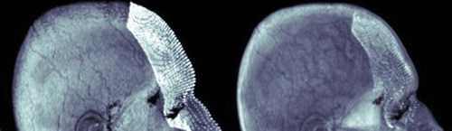
As can be observed from Figure 1, two regular grids of the same size are extracted from the outer and the inner surfaces of the forehead soft tissue layer. Thus, a soft tissue volume is obtained as a grid of U × V × 2 points.

2.1.2. Volume spline fitting

A volume spline of M × N × 2 (e.g. 5 × 5 × 2) control points, where M ≤ U and N ≤ V, is fit to the U · V · 2 points of the segmented grid. The general volume spline equation can be written as follows: (1)

Here, V(u, v, w, B) is the 3D position of a point inside the volume in general coordinates (u, v, w), B_a,b,c's are the 3D control points of the volume spline, and N...(⋅)'s are the basis functions. Using the notation in 7, we may combine the basis functions in the Jacobian vector and represent (1) in matrix form as follows: (2)

Here, B is a matrix of size (M · N · 2) × 3, representing the control points in general coordinates: (3) J is a vector of size M · N · 2: (4)

Then, by putting all the points in matrix notation, we obtain (5)

Here, V is the matrix of data points: (6)

Finally, C is the matrix of Jacobian vectors for data points. C has the size of (U · V · 2) × (M · N · 2) (7)

As U · V · 2 ≥ M · N · 2 and the rank of C is maximal (i.e. equal to M · N · 2), the control points covering the given volumetric data are computed by using the pseudo inverse of C based on the least squares estimation: (8)

2.2. Dynamic modelling

The dynamic behaviour is introduced to the volume spline model based on the DNURBS physics 7. It is established on the work–energy version of the Lagrangian dynamics. The control points of the DNURBS are considered as localized masses having localized stiffness and damping which are related to all parts of the surface via the Jacobian defined in (4). Consequently, the equation of motion in terms of control points is defined as follows: (9)

In this equation, T(t) is the total kinetic energy of the system, U(t) the total elastic potential energy of the system, F_R(t) Raleigh's dissipation energy, f(u, v, w) the external force applied to the system and B(t) the control points in general coordinates as a function of time. In this study, we have the same equation to identify the dynamics of motion for the control points of our model. Furthermore, the elastic and dissipation energies are defined as the stiffness and damping matrices as in 7 also. However, in 7 these were defined for dynamic surfaces, whereas in our model we use volume splines. Thus, triple integrals are computed for the three orthogonal parameter values u, v and w. The kinetic energy for the model is defined as follows: (10)

Here μ(u, v, w) is the mass density function defined over the orthogonal (u, v, w) parameter space and is the time derivative of the points inside the spline volume. When the derivatives on both sides of (5) are taken, the following equation is obtained as J is obtained from the basis functions and it is not a function of time: (11)

Then, T can be written as follows: (12) where M is (13)

Here, M is a matrix of size (M · N · 2) × (M · N · 2), which represents localized mass for each control point and covariant relation of mass distribution among the control points.

Similarly, using the dissipation energy F_R(t), we obtain the (M · N · 2) × (M · N · 2) damping matrix D which represents the localized damping coefficients of the control points and the covariant relation of energy loss among them: (14) (15) Here, γ(u, v, w) is the damping density function defined over the parameter space.

In 7, the energy model of a thin plate under tension is adopted as an elastic potential energy model for DNURBS surfaces, i.e. for two dimensions. Here, this definition is adapted to three orthogonal dimensions as follows: (16)

Correspondingly, K is a matrix of size (M · N · 2) × (M · N · 2), which represents localized elastic relations among the control points. Furthermore, α(u, v, w) and β(u, v, w) are the elasticity (stiffness) functions which control local tension and rigidity, respectively. By denoting J_x as the first derivative of J with respect to x and J_xy as the second derivative with respect to x and y, K can be calculated as follows: (17)

Finally, Equation (9) can be rewritten in matrix form as follows: (18) where F_B(t) is the generalized force vector, obtained through the principle of virtual work done by the applied force distribution f(u, v, w): (19)

Furthermore, I(t) is the mass moment of inertia, which happens to be zero, as the time derivative of J is zero. (20)

Thus, the final equation of motion can be written as follows: (21) which can be written as a system of differential equations (22)

This system of differential equations can be solved through time starting from an initial state. If the initial state is the resting state before the application of force, then the initial will be the initial locations of the control points of the volume and the initial will be zero. Starting from this initial state, the positions of the control points through time can be computed when an external force is applied to the model. When the model reaches the steady state eventually, the volume will have its final shape. The new surface model can be obtained from the new positions of the control points by (1).

3. Literature for skin physical properties

There are many in vivo force–displacement experiments in the literature, which are designed to obtain the biomechanical parameters of human skin 8–15. Most of them are applied to the human thigh and forearm, where muscle mechanical parameters interfere with the skin parameters. There are no studies performed on human facial skin.

Not only the experiment styles but also the parameter values vary among studies. The parameters are different for various regions of the human body and also different from person to person. Although human skin is heterogeneous and anisotropic, most of the studies model human skin as linear and uniform 8, especially when a very small force is applied to the skin. In this study, skin behaviour is also studied for very small forces and the linear model is used with uniform parameters.

As it is hard to obtain skin biomechanical properties in vivo, only a limited number of parameters such as stiffness are estimated in the literature. The stiffness (α and β in Equation (17)) and damping coefficient (γ in Equation (15)) values for forearm, thigh and scalp skin range between 12–750 N m⁻¹ and 0.08–350 Ns m⁻¹, respectively 8–14. The mass density (μ in Equation (13)) for skin is given approximately as 1100 kg m⁻³ 13.

4. Experiment for the acquisition of 3D facial skin deformation

A very small force is applied on the forehead skin surface. The measurements of the applied force and the deformation occurred on the surface are calculated by a force sensor and multiple cameras, respectively. By performing stereo analysis between the stereo images, 3D shapes of the surfaces before and after the application of force are obtained by 3D reconstruction. In this section, all the experiment steps are summarized.

4.1. Experiment setup and data collection

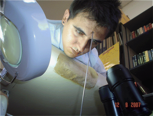
There are mainly four classes of equipment. They are multiple cameras required for imaging, the force sensor and the data collector device required for force measurement, the equipment required to keep the subject's head fixed and the equipment required for lighting the experimental environment.

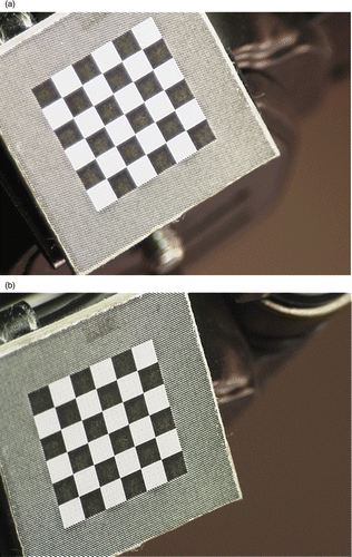
The colour cameras with 1024 × 768 resolution (Sony DFW-X710) are connected to a single tripod and positioned so that they all clearly see the experimented part of the skin without any occlusion (Figure 2a). The cameras are calibrated using the calibration images (Figure 3) by the method proposed in 31,32 at the beginning and fixed throughout the experiment.

Figure 2. (a) The cameras and the force sensor probe positioned on a tripot. (b) The force sensor, the probe and the measurement device.

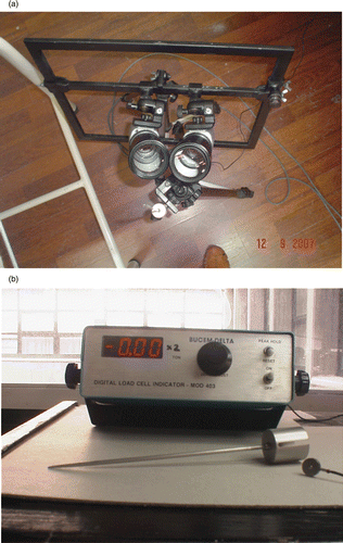
Figure 3. Calibration images.

As a very small amount of force is applied on the skin, a very precise and sensitive force sensor is used and located altogether with the cameras (Figure 2a). As the area of the force sensor is big (1.5 cm in diameter), it occludes the view and thus the cameras cannot see the actual deformation. Thus, a very thin but strong probe is placed over the sensor keeping the friction minimal. In Figure 2(b), the force sensor, the probe and the measuring device (BUCEM DELTA Digital Load Cell Indicator Mod 403) are shown. The force sensor and the data collection device are calibrated using small weights of known values.

During the experiment, various force values are applied to the surface. The force value is recorded when the measurement becomes stable for a couple of seconds on the device's screen. Simultaneously, the corresponding stereo images are captured and stored (Figure 4). The stereo images of the resting surface are also recorded before the application of force (Figure 4).

Figure 4. Stereo images collected when force is not applied (a and b) and when force is applied (c and d).

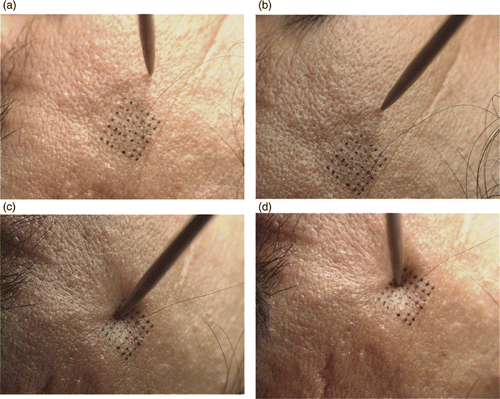
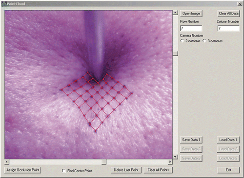
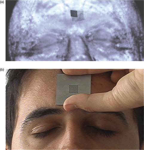
In order to obtain the 3D shape information of the surface, corresponding image points between the stereo pair are matched. To find the correct corresponding pairs, the experimented surface is marked with regular grid points before the experiment. A metal sheet with 7 × 7 holes, which have radius of 0.5 mm and are located 1.5 mm apart, is used to mark the surface using an appropriate pen (Figure 5). This process is completed very carefully in order not to let the marks diffuse on the surface. Matching between the stereo pair can also be done automatically by various methods but this is out of the scope of this article. Instead, we manually match the grid of marks by a user interface given in Figure 6. The grid on the face and the user interface are also helpful in localizing the contact point and the direction of the force from the images.

Figure 5. Marking on the face by the metal grid.

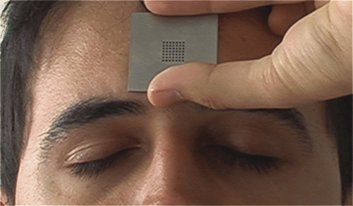
Figure 6. Graphical user interface of the programme, which is used to label the points on the surface, the contact point and the direction of the force.

In order to have minimal frictional force, the force should be applied on the surface in normal direction upright from the floor. Thus, the subject is placed on a stricter facing the floor while the neck of the subject is held still and fixed. In Figure 7, the subject is seen while a very small force (370 mN) is applied on the forehead. As the applied force is very small, only the soft tissue of the face is deformed and the head is not moved.

Figure 7. Position of the patient while a small force is applied on the forehead.

4.2. 3D surface reconstruction

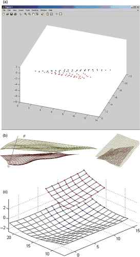
First of all, the corresponding points on the image pair are matched. Also, the location of the force contact is labelled. These are done manually using the labelling tool (Figure 6). Then, the surface is obtained as a 3D point cloud by reconstructing the point pairs (Figure 8a). This is done for the stereo pairs recorded before and after the force application. In this way, it becomes possible to measure the difference between the locations of the points before and after the force application. When a spline surface is fit to the point cloud 33, the difference between the surfaces can also be computed. In Figure 8(b), the spline surfaces for the point clouds are shown. Actually, the reconstructed part of the surface is one-fourth of the whole deformed surface because only the part which is not occluded is considered. To obtain the whole deformed surface, the symmetries of this part are combined and the whole deformed surface is approximated as shown in Figure 8(c).

Figure 8. (Available in colour online) (a) 3D point cloud for the surface before (blue) and after (red) the force application. (b) Different views of the spline surfaces fit to the point cloud surfaces. Yellow is the initial surface (before force application) and red is the deformed surface (after force application). (c) The whole deformed surface obtained from the one-fourth. The smaller mesh (red dots) is the reconstructed shape. The whole deformed surface (the bigger mesh) is approximated by the symmetries of the reconstructed mesh.

4.3. Collected data

The experiment is performed for force values between 60 and 270 mN at 30 mN intervals. Each force value is applied 10 times at different points on the experimented forehead region. The reconstructed surfaces at each 10 measurements are averaged to obtain noise-free surface information for each applied force value. For example, in Figure 9, the initial and the final surfaces are shown when 270 mN is applied. The amount of deformation is given in grey level.

Figure 9. The actual initial surface (a) and the actual final surface (b) when 270 mN is applied on the forehead.

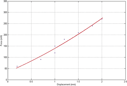
The amount of indentation only in the normal direction and only at the point of force application is measured for different force values and a force–displacement curve is obtained where the slope becomes 60 N m⁻¹ (Figure 10). This value is consistent with the literature where 12 10, 30 9 and 50 N m⁻¹ 11 are given for the forearm and 300 N m⁻¹ 13 is given for the human scalp. Also, the linear relationship between the applied force and the amount of indentation is consistent with the literature as for small forces the skin acts like a linear material 8–14.

Figure 10. Force versus displacement plot where the slope is 60 N m⁻¹.

5. Forward solution of the model

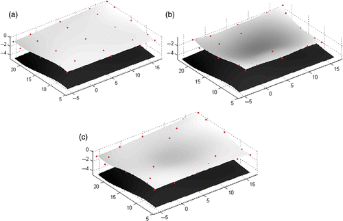
The skin volume is segmented from the MR data of the patient. A 15 × 20 × 2 mm³ part of the skin volume is modelled by a volume spline with 5 × 5 × 2 control points (Figure 11(a)). The lower surface of the model is fixed because it sits on a rigid structure, i.e. on the forehead bone. Also, bigger stiffness values are used for the edge regions of the model in order to prevent the model collapse. This can be thought of as the model being smaller part of a larger skin area.

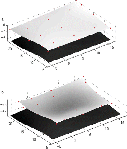
Figure 11. Shape of the skin volume outer surface at rest (a) when 300 mN (b) and 1000 mN (c) is applied in the direction pointed by the arrow. Red dots are the control points of the volume spline model.

As the only value found in the literature for the skin mass density is 1100 kg m⁻³ (Section 3), it is used as the mass density throughout this study. The duration for the model to reach the steady state and the behaviour of the model during transient response depend on the damping parameter. But, the final steady state of a second-order dynamical system such as ours will be independent of the damping coefficient. In other words, while the small displacement on the facial skin is being computed when a force is applied, the value of the damping coefficient will affect the transient state but it will have no effect on the final steady state shape 34. As we are not interested in the behaviour of the model through time but in the final shape of the model only, time-independent behaviour of the model is investigated. The only important thing is to use an appropriate damping value so that our system will reach the steady state in the shortest time. We have found that the values between 1 and 30 Ns m⁻¹ can be used as appropriate values for the damping coefficient (which is also consistent with the literature given in Section 3) by trial and error.

The forward solution of the model is performed for various different stiffness coefficient values. In the rest of this section, results are shown when 24 N m⁻¹ is used for α and 0 is used for β stiffness coefficients (17). The model is solved by using Equation (22) when a small virtual force is applied in the middle of the upper surface. The solution is implemented by the differential equation solution functions (i.e. ode45) of MATLAB version R2008a. Starting from the initial state of rest, the model is solved through time until the model reaches the steady state. The steady state condition is checked by observing the magnitude of the transient oscillations. When the magnitude of the oscillation drops to 5% of the initial highest oscillation magnitude, the system is considered to reach the steady state 34. This usually takes 10 ms when MATLAB is run on a 2.2 GHz double core laptop.

When a small force is applied on the upper surface of the model, the upper surface bends and the volume is deformed. As the lower surface is fixed, there is no deformation on it. In Figure 11, the surface shape and the control point locations are shown when the tissue is at rest (initial state) and when 300 and 1000 mN forces are applied on the model (final steady states).

6. Parameter estimation by the inverse solution of the model

6.1. Introduction

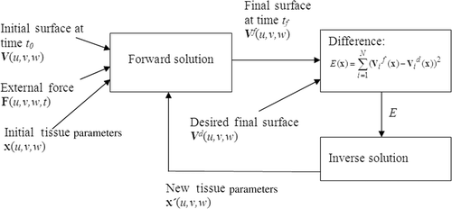
The inverse solution is to estimate the model parameters when the initial and the final shapes of the model surface and the applied force are known. In this study, the initial shape is the shape reconstructed during the experiment before the force is applied. The skin volume at the experimented region is obtained by the segmentation of the MR data. The surfaces obtained during the experiment and the volume segmented from the MR data are registered manually (Figure 12). The final shape is the shape reconstructed during the experiment after the force is applied on the face. This is called the desired final surface in order to distinguish it from the final shape of the model when the forward solution of the model is obtained with some parameter values starting from the initial shape.

Figure 12. Marking on the face and the face MR data registered to the marked face region.

There is no closed form inverse solution for the model and some iterative optimization methods are needed. In Figure 13, the steps of the iterative inverse solution are visualized. In the inverse solution, first of all, the forward solution of the model is obtained for the applied force value starting from the initial shape (V) and using some initial values for the parameters. Then, the difference between the final shape, obtained from the steady state of the forward solution (V^f), and the desired shape, obtained during the experiment (V^d), is employed as the objective function (23), which needs to be minimized. The parameter values are updated so that the objective function is minimized. Then, the new parameter values are employed in the forward solution. This iteration continues until the final shape of the model becomes very close to the desired final shape (i.e. the objective function value becomes smaller than 10⁻⁶) or the maximum number of iterations (i.e. 1100) is exceeded.

Figure 13. Forward and inverse solution steps.

The objective function is computed as the sum of squared distance between corresponding surface points, namely between the final surface and the desired surface: (23)

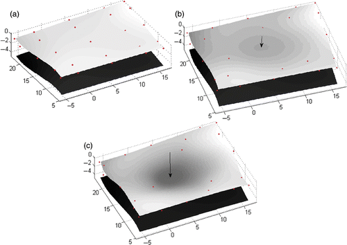
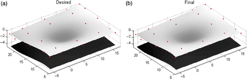
Here, x is the parameter vector of our volume spline-based dynamic model and i the index for the surface points, where N is the total number of surface points (i.e. U · V). For example, in Figure 14(a) and (b), the initial surface before the application of force and the desired surface obtained during the experiment, when 270 mN is applied on the actual face, are shown, respectively. In Figure 14(c), the result of the forward solution of the model is shown when 270 mN is applied on the model surface and 1100 kg m⁻³, 50 N m⁻¹, 24 Ns m⁻¹ are used as mass density, stiffness (α) and damping coefficients, respectively. The difference between the desired and the final surfaces (i.e. E) for this case is 12.25. If the appropriate model parameters had been used in the forward solution of the model, then this difference would have been very close to zero.

Figure 14. (a) The inital surface before the application of force, (b) the desired facial surface and (c) the result of the forward solution of the model when 1100 kg m⁻³, 50 N m⁻¹, 24 Ns m⁻¹ are used as mass density, stiffness and damping coefficients.

In the following sections, first of all, least squares optimization is explained. Then, the inverse solution based on the least squares is applied to simulations. Finally, the inverse solution is employed to the real data.

6.2. Nonlinear least squares estimation

The explanations of this subsection are based on 35–39. The function (23) can be represented in vector denotation as follows: (24) where V is the vector-valued function and the factor 1/2 serves for a more convenient normalization of the derivatives. Here (i = 1, 2, …, N). In fact, by the chain rule we obtain 39 (25)

The Hessian of E can be derived by differentiating with respect to the coordinates x_j: (26)

Let be a solution of (24) and suppose . Then, , i.e. all the residuals r_j are vanishing and the model fits data without error 35. As a result, and, thus, , which confirms our first-order necessary optimality condition. Furthermore, we can obtain the Hessian of E being which is a positive semi-definite matrix at the solution. If, additionally, is a matrix with full rank, i.e. then is positive definite. Hence, a second-order necessary optimality condition is provided such that is also a strict local minimizer 35. Based on this basic idea, a number of specialized nonlinear least squares methods originate. The simplest of these methods, called Gauss–Newton uses this approximate description in a direct way. It makes a replacement of the Hessian in the formula (27) such that we have a relation (28) where q is Gauss–Newton increment If and then, near the solution , Gauss–Newton's method behaves like Newton's 35. But, we need not pay the computational cost of calculating second derivatives. Gauss–Newton's procedure sometimes behaves poor if there is one or a number of outliers, i.e. if the model does not fit the data well, or if is not of full rank p. In these cases, there is a weak approximation of the Hessian. In fact, many other methods for nonlinear least squares can be understood as using some approximation to the second additive term in formula (26) for the Hessian, i.e. of (29)

The simplest of these approximations is (30) with some scalar λ ≥ 0. This approximation yields the following linear system: (31)

This is referred to as Levenberg–Marquardt method 40,41. We can often find this method implemented in the context of a trust–region strategy. These methods were first applied to solve nonlinear least squares problems and then they have been adapted to more general optimization programmes 39,42. The size of the step, q, is obtained by minimizing a quadratic model of the objective function with Gauss–Newton approximation to the Hessian: (32)

This is a constrained optimization problem. The optimality conditions for this programme show that q will be the solution of the linear system where λ ≥ 0 is a scalar, is positive semi-definite and

If is positive definite and Δ is sufficiently large, then the solution of the (32) is the solution to the Newton equations. Without these assumptions, the method guarantees that if and

Hence, q is a function of λ and, indirectly, a function of Δ 39. The scalar Δ can be chosen in the set of positive numbers, based on the effectiveness of the Gauss–Newton method.

The Levenberg–Marquardt method can be understood as a compromise between both the Gauss–Newton (if λ ≈ 0) and the steepest-descent method (if λ is very large) 39. An adaptive and sequential way of choosing λ and, by this, of the adjustment of mixture between the methods of Gauss–Newton and steepest-descent, is presented in 39. Let us note that can also be seen as a regularization term that shifts the eigenvalues of away from 0. Another way to solve the system (31) for given , i.e. to find the (k + 1)-th iterate , consists in an application of least squares estimation. If we denote (33) by , where and , then we can study the regularized problem by adding to the squared residual norm a penalty or regularization term of the form , i.e. (33) where L may be the unit matrix, but it can also represent a discrete differentiation of first or second order. This regularization serves to diminish the complexity of the model 42.

6.3. Inverse solution for the simulations

In this section, the inverse solution of a simulation is performed to make sure that the solution works correctly. First of all, forward solution is computed for a given model parameter set and a given force value, starting from the initial model shape. As the uniform mass density, damping, vertical (α_w) and horizontal (α_u and α_v) stiffness coefficients, the values 1100 kg m⁻³, 24 Ns m⁻¹, 5 and 0.1 N m⁻¹ are used, respectively. The final shape is computed when 300 mN is applied on the surface of the model. This final shape is also used as the desired shape and inverse solution is solved based on it. Parameter estimation is performed only for the stiffness coefficients.

The function (23) can be considered as a nonlinear least squares curve fitting problem. The optimization process is implemented by the Lsqnonlin function of the MATLAB optimization toolbox. The function solves nonlinear least squares curve fitting problems of the form given in (23). It uses the Gauss–Newton 36 or Levenberg–Marquardt method 40,41 with polynomial line search strategies. The selected termination conditions for iterations are the tolerance on E and the variable values (i.e. 10⁻⁶) and the maximum iteration number (i.e. 1100).

Beginning from various initial stiffness values, the inverse solution is computed. The estimated stiffness values and the corresponding E values are given in Table 1 for various initial values. Also, the durations of the inverse solution are given in the table. For nearly all initial values, the actual values are estimated if the iterations are continued long enough. For example, when the inverse solution iterations are started with initial values of 50 and 40 for the horizontal and vertical stiffness coefficients, after 1751 s the estimated values become 12.4368 and 5.0215, but after 4090 s the estimated values become 0.10063 and 5.012, which are very close to the actual values (i.e. 0.1 and 5). These results are shown in the last two lines of Table 1.

Table 1. Estimated parameter values for different initial values where the true values are 0.1 and 5 N m⁻¹ for the horizontal and the vertical stiffness, respectively.

Initial α horizontal (N m^−1)	Initial α vertical (N m^−1)	Duration of inverse solution (s)	Estimated α horizontal (N m^−1)	Estimated α vertical (N m^−1)
1	10	1831	0.1243	5.0001
7	7	1758	0.11366	5
12	23	1104	0.10026	5
50	40	1751	12.4368	5.0215
50	40	4090	0.10063	5.012

6.4. Inverse solution for the experimental data

The inverse solution is applied to the experimental data as follows. The surfaces reconstructed before and after the force application during the experiment are used as the initial and the desired surfaces in the inverse solution for the corresponding force value. The mass density and the damping coefficient values are set as 1100 kg m⁻³ and 1 Nm s⁻¹, respectively. The inverse solution is performed for the horizontal and the vertical stiffness coefficients (α) where the parameters β are assumed to be zero. The desired surface (obtained during the experiment) and the final surface (obtained at the end of parameter estimation iterations) are shown in Figure 15 when the objective function value is 9 × 10⁻⁶. The mean of the resultant estimated values for different data sets are found to be 80 and 2 N m⁻¹ for the vertical and the horizontal stiffness coefficients, respectively.

Figure 15. The desired surface obtained during the experiment (a) and the final surface obtained by the parameter values estimated after the inverse solution (b) when the objective function value becomes 9 × 10⁻⁶ at the end of optimization iterations.

When compared with the literature values (Section 3), these values are consistent. In the literature, the values given for the vertical stiffness coefficient varies between 12 and 750 N m⁻¹. When the force–displacement curve is computed for the experimental data for only the data collected at the point of force application, we calculated the slope of the curve as 60 N m⁻¹ (Section 4.3, Figure 10). When the stiffness parameter is estimated by the inverse solution of the dynamic volume spline where the whole deformation is considered, 80 N m⁻¹ is found to be the best value for the model to represent the actual tissue behaviour.

7. Facial animation

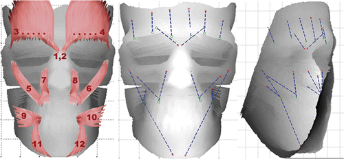
We model segmented facial soft tissue volume (i.e. the skin layer over the muscle layer) by the dynamic volume spline method where the surface of the muscle layer is considered as the rigid boundary. The origin and the insertion points of the muscles are used to decide on the directions of the applied forces on the soft tissue model. But, instead of force application, muscle attachment points are displaced to simulate facial muscle contractions. The displacement vector is from the muscle insertion point towards the origin point (Figure 16). The magnitude of the muscle contraction is controlled by the magnitude of this displacement. When the muscle insertion point is displaced, this disturbs the energy equilibrium in the soft tissue model and the model relaxes accordingly due to its elastic behaviour. When the model reaches its steady state after the disturbance, the facial expression is simulated.

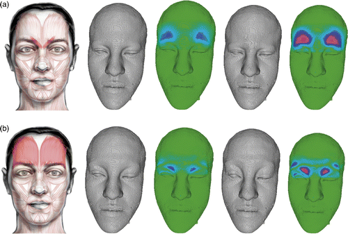
Figure 16. (Available in colour online). (a) Facial muscles, namely corrugator (1, 2), frontalis (3, 4), zygomatic major (5, 6), caninus (7, 8), risorius (9, 10) and triangularis (11, 12), are shown over the segmented skull. (b) Muscles are shown as linear vectors emerging from the origin points (red crosses) towards the instertion points (green circles) on the inner soft tissue layer. (c) The muscle vectors are depicted inside the inner soft tissue layer.

The animation results for frontalis and corrugator muscles are shown in Figure 17. Each row includes a muscle's animation where the muscle's placement on the face 43, the animation results of our model for two different degrees of contraction (first less than more) and the difference between the resting face model and the animated face model are given in the columns from left to right. In the difference faces, zero difference is coloured green and the colour changes to blue and red as the difference increases.

Figure 17. (Available in colour online). Facial expression simulation by the contraction of (a) frontalis and (b) corrugator muscles. For each muscle, two different degrees of contraction (first less, then more) are given. The difference between the resting face model and the animated face model is also depicted in colour scale. Green–ındifferent, blue–moderately different and red–most different.

8. Conclusion

In this study, human facial soft tissue is modelled by a dynamic volume spline and the parameters of this model are estimated from the actual human facial skin properties by the optimization-based inverse solution. Based on our preliminary research 25, the dynamic volume spline model is used for soft tissue modelling and especially for human facial skin modelling. Also, optimization-based inverse solution is applied to the dynamic volume spline. The model and the inverse solution are applied to a very small area on the forehead and the estimated parameters are used to model the whole face and the face model is applied for facial animation.

The main purpose of the parameter estimation by inverse solution is to obtain a realistic model so that the model will behave in a similar way to the actual facial soft tissue. The proposed model is a physical and mechanical model and the model parameters correspond to the real tissue parameters such as mass density, elasticity (stiffness) and damping. Different values are presented in the literature for human skin physical properties because these vary among people and body parts. In this study, we estimate them for the dynamic spline model and see that with the estimated parameter values the model behaves in a very similar way to the actual tissue characteristic which is obtained during the force–displacement experiment.

The model is used with uniform parameters where the literature value 1100 kg m⁻³ is used for the mass density and an appropriate value (i.e. between 1 and 30 Ns m⁻¹) is used for the damping coefficient. The stiffness coefficients (α) in all three dimensions (vertical axis and horizontal plane) are estimated by the inverse solution when the rest of the parameters are set to zero. The estimated values for the vertical and the horizontal stiffness coefficients are found to be 80 and 2 N m⁻¹, respectively. The stiffness values given in the literature vary from 12 to 750 N m⁻¹. These values are given for a single direction and dimension (normal to the surface) and obtained when the force–displacement relation is considered only for the point of force application. However, in the inverse solution of the dynamic volume spline, the whole deformation around the point of force application is considered and a dynamic volume model is solved to estimate the parameter values.

Our mathematical treatment allows a multiparameter estimation problem and it will in future host an even further parametrically extended problem of that kind. We developed various refined techniques of parameter estimation, e.g. based on generalized additive models 44 and multivariate adaptive regression spline (MARS) and CMARD 45 and received very good results. In fact, all our procedures are well regularized. These kinds of regularizations are first steps towards the overcoming of singularities. We refer to 46 for a survey on a singularity in a possibly highly nonlinear and high dimensional optimization. Together with differential topology around the point of applied force, the singularity could be faced even better. We note that with respect to the uncertainties remaining, we are using robust optimization, we develop a robust variant of our MARS version (CMARS) and have worked out regression models with interval uncertainty and, more satisfactory, ellipsoidal uncertainty 47. This article may, therefore, also serve for an invitation of the interested readers in participating in these future investigations.

The most important issue is the similarity of the estimated behaviour with the actual tissue behaviour and this is achieved by the model with the estimated parameter values. With these estimated parameters, the model gets the same final shape as the actual tissue under the same force conditions. We perform parameter estimation only for α coefficient in three dimensions and we leave the parameter estimation for all parameters of the model as a future study.

The data used in the inverse solution is obtained by a force–indentation experiment. In the literature, there are force–displacement experiments where indentation is measured only at the force contact point. In these experiments, a very simple and 1D dynamic equation is used to model soft tissue and the model parameters are estimated from the experimental data by simple matrix inversion techniques. In this study, a new force–displacement type of experiment is proposed where the whole deformation which occurs on the tissue after the application of force can be measured. This is done by imaging the experimented area by stereo cameras and obtaining the surface shape by 3D reconstruction. The most important thing here is to match corresponding points between the stereo image pairs and this is done with the help of marking a grid of points on the face. Such a grid of points also helps in registering the surfaces reconstructed before and after the application of force and also in registering the subject face and the model. Automatic matching of corresponding points in the stereo images could also have been done but this is left as a future study.

When the whole surface deformation information, instead of the displacement information at a single point, is available, the parameters of a very complex model such as the dynamic volume spline can be estimated better. It is highly complex to model a material such as the human face which has an anisotropic, heterogeneous and nonlinear elasticity. There is not a model yet which models the living tissue completely in terms of simulation quality and computation speed. Although with the linearity and uniformity assumptions, the proposed dynamic volume spline model is promising in terms of visual quality and computation complexity. Because, when the appropriate parameters are used, we can obtain the same model shapes as the shapes we obtained during the experiments. Also, although the structure of the model and the types of equations solved are very similar to FEMs, as the dynamic volume spline model is based on splines and is solved for control points only, less number of computations are performed when compared with FEM, which partitions the whole volume into small volumes and perform the computations for each of them.

Finally, 3D human facial soft tissue is segmented from 3D MR data and is modelled by the dynamic volume spline where the parameters estimated in this study are used. The face model is animated for some forehead expressions by displacing the muscle attachment points on the soft tissue volume. The dynamic model responds to such a displacement, relaxes and obtains its final shape.

Acknowledgements

This study is partially supported by TUBITAK 105E128 and BAP-2008-03-01-04.

References

- Sedef, M, Samur, E, and Başdoğan, Ç, 2006. Real-time finite-element simulation of linear viscoelastic tissue behavior based on experimental data, IEEE Comput. Graph. Appl. 26 (2006), pp. 58–68.
- Debunne, G, Desbrun, M, Cani, MP, and Barr, AH, 2001. "Proceedings of Siggraph". In: Dynamic Real-time Deformations Using Space & Time Adaptive Sampling. New York: ACM Press; 2001. pp. 31–36.
- Hauth, M, Groß, J, and Straßer, W, 2003. Interactive physically based solid dynamics, Proceedings of Eurographics/Siggraph Symposium on Computer Animation. San Diego, CA: Eurographics Association; 2003. pp. 17–27.
- Schoner, JL, Lang, J, and Seidel, HP, 2004. Measurement-based interactive simulation of viscoelastic solids, Comput. Graph. Forum 23 (2004), pp. 547–556.
- Schwartz, JM, Denninger, M, Rancourt, D, Moisan, C, and Laurendeau, D, 2005. Modeling liver tissue properties using a non-linear visco-elastic model for surgery simulation, Med. Image Anal. 9 (2005), pp. 103–112.
- Delingette, H, , Towards realistic soft tissue modeling in medical simulation, INRIA. Report No 3506. September 1998. http://www.inria.fr/Equipes/EPIDAURE-eng.html.
- Qin, H, and Terzopoulos, D, 1996. D-NURBS: a physics-based framework for geometric design, IEEE Trans. Visual. Comput. Graph. 2 (1996), pp. 85–96.
- Duchemin, G, Maillet, P, Poignet, P, Dombre, E, and Pierrot, F, 2005. A hybrid position/force control approach for identification of deformation models of skin and underlying tissues, IEEE Trans. Biomed. Eng. 52 (2005), pp. 160–170.
- Boyer, G, Zahouani, H, Bot, ALe, and Laquieze, L, , In vivo characterization of viscoelastic properties of human skin using dynamic micro-indentation, Proceedings of 29th Annual International Conference of the IEEE EMBS, Lyon, France, 2007..
- Pailler-Mattei, C, Bee, S, and Zahouani, H, 2008. In vivo measurements of the elastic mechanical properties of human skin by indentation tests, Med. Eng. Phys. 30 (2008), pp. 599–606.
- Pailler-Mattei, C, Nicoli, S, Pirot, F, Vargiolu, R, and Zahouani, H, 2009. A new approach to describe the skin surface physical properties in vivo, Colloids Surf. B 68 (2009), pp. 200–206.
- Tran, HV, Charleux, F, Rachik, M, Ehrlachers, A, and Ho Batho, MC, 2007. In vivo characterization of the mechanical properties of human skin derived from MRI and indentation techniques, Comput. Meth. Biomech. Biomed. Eng. 10 (2007), pp. 401–407.
- Gambarotta, L, Massabo, R, Morbiducci, R, Raposio, E, and Santi, P, 2005. In vivo experimental testing and model identification of human scalp skin, J. Biomech. 38 (2005), pp. 2237–2247.
- Gennison, J, Baldeweek, T, Tanter, M, Catheline, S, Fink, M, Sandrin, L, Cornillon, C, and Querleux, B, 2004. Assessment of elastic parameters of human skin using dynamic elastography, IEEE Trans. Ultrason. Ferroelectric Freq. Contr. 51 (2004), pp. 980–990.
- Bischoff, JE, Arruda, EM, and Grosh, K, 2000. Finite element modeling of human skin using an isotropic, nonlinear elastic constitutive model, J. Biomech. 33 (2000), pp. 645–652.
- Arruda, EM, and Boyce, MC, 1992. A three-dimensional constitutive model for the large stretch behavior of rubber elastic materials, J. Mech. Phys. Solids 41 (1992), pp. 389–412.
- Duchemin, G, Maillet, P, Poignet, P, and Dombre, E, 2005. A hybrid position/force control approach for identification of deformation models of skin and underlying tissues, IEEE Trans. Biomed. Eng. 52 (2005), pp. 160–170.
- d’Aulignac, D, Laugier, C, and Cavusoglu, MC, 1999. Towards a realistic echographic simulator with force feedback, Proceedings of the IEEE-RSJ International Conference on Intelligent Robots and Systems. Vol. 2. 1999. pp. 727–732.
- Gao, H, Chui, C, and Lee, J, 1992. Elastic contact versus indentation modeling of multi-layered materials, Int. J. Solids Struct. 29 (1992), pp. 2471–2492.
- Bec, S, Tonck, A, Georges, JM, Georges, E, and Loubet, JL, 1996. Improvements in the indentation method with a surface force apparatus, Philos. Mag. A 74 (1996), pp. 1061–1072.
- Rar, A, Song, H, and Pharr, GM, 2002. Assessment of new relation for the elastic compliance of a film-substrate system, Mater. Res. Soc. Symp. Proc. 695 (2002), pp. 431–436.
- Perriot, A, and Barthel, E, 2004. Elastic contact to a coated half-space: effective elastic modulus and real penetration, J. Mater. Res. 19 (2004), pp. 600–608.
- Diridollou, S, Black, D, Lagarde, JM, Gall, Y, Berson, M, Vabre, V, Patat, F, and Vaillant, L, 2000. Sex- and site-dependent variations in the thickness and mechanical properties of human skin in vivo, Int. J. Cosmet. Sci. 22 (2000), pp. 421–435.
- Ulusoy, I, Akagunduz, E, and Weber, GW, , Estimation of parameters for dynamic volume spline models, Proc. Int. Conf. Eng. Optim. (2008), Inverse Problems in Science and Engineering (2010), DOI: 10.1080/17415971003624371..
- Tasdizen, T, Weinstein, D, and Lee, JN, , Automatic tissue classification for the human head from multispectral mri, Tech. Rep. UUSCI-2004-001, University of Utah, Utah, 2004..
- BioPSE, Problem solving environment for modeling, simulation, and visualization of bioelectric fields, Scientific Computing and Imaging Institute (SCI). Available at http://software.sci.utah.edu/biopse.html, 2002..
- Bet. Available at http://www.fmrib.ox.ac.uk/analysis/research/bet/slideshow/index.html.
- Brainsuite. Available at http://www.loni.ucla.edu/Software/BrainSuite2.
- Koch, RM, Gross, MH, Carls, FR, von Buren, DF, Fankhauser, G, and Parish, Y, , Simulating facial surgery using finite element methods, Proceedings of ACM Siggraph, 1996, pp. 421–428..
- Zhang, Z, 2000. A flexible new technique for camera calibration, IEEE, T. Pattern Anal. 22 (11) (2000), pp. 1330–1334.
- Camera calibration toolbox for Matlab. Available at http://www.vision.caltech.edu/bouguetj/calib_doc.
- Piegl, L, 1991. On NURBS: a Survey, IEEE Comput. Graph. Appl. 11 (1991), pp. 55–71.
- Ogata, K, 1990. Modern Control Engineering, . Englewood Cliffs, NJ: Prentice-Hall International Edition; 1990. p. 260.
- Nash, G, and Sofer, A, 1996. Linear and Nonlinear Programming. New York: McGraw-Hill; 1996.
- Dennis, JE, "Nonlinear least-squares". In: Jacobs, D, ed. State of the Art in Numerical Analysis. London: Academic Press; pp. 269–312.
- Taylan, P, and Weber, G-W, 2008. Organization in finance prepared by stochastic differential equations with additive and nonlinear models and continuous optimization, Organizacija (Organization J. Manag. Info. Sys. Hum. Resources) 41 (2008), pp. 185–193.
- Aster, A, Borchers, B, and Thurber, C, 2004. Parameter Estimation and Inverse Problems. London: Academic Press; 2004.
- Kürüm, E, Yildirak, K, and Weber, G-W, , A classification problem of credit risk rating investigated and solved by optimization of the ROC curve, preprint at IAM, METU, Eur. J. Oper. Res., submitted for publication..
- Levenberg, K, 1994. A method for the solution of certain problems in least-squares, Q. Appl. Math. 2 (1994), pp. 164–168.
- Marquardt, D, 1963. An algorithm for least-squares estimation of nonlinear parameters, SIAM J. Appl. Math. 11 (1963), pp. 431–441.
- Weber, G-W, Taylan, P, Yildirak, K, and Görgülü, ZK, , Financial regression and organization, to appear in the Special Issue on Optim Finance DCDIS-B..
- Flores, VC, , Artnatomy/Artnatomıa. Available at www.artnatomia.net, SPAIN, 2005..
- P. Taylan, G.-W. Weber, and A. Beck, New approaches to regression by generalized additive models and continuous optimization for modern applications in finance, science and technology, in the special issue of Optimization in honour of Prof. Dr. A. Rubinov, B. Burachik, and X. Yang, guest eds., 56, 2007, pp. 1–24..
- Jongen, HTh, and Weber, G-W, 1990. On parametric nonlinear programming, Ann. Oper. Res. 27 (1990), pp. 253–284.
- Weber, G-W, Batmaz, I, Köksal, G, Taylan, P, and Yerlikaya-Özkurt, F, , CMARS: A new contribution to nonparametric regression with multivariate adaptive regression splines supported by continuous optimisation, Adv. Comput. Appl. Math, submitted for publication..
- G.-W. Weber, Ö. Defterli, S.Z. Alparslan Gök, and E. Kropat, Modeling, inference and optimization of regulatory networks based on time series data, invited paper, Eur. J. Oper. Res., submitted for publication..