Discrete variational adjoint assimilations for parameter optimizations via spectral methods

Abstract

In this article, we investigate the parameter optimization problem via the variational adjoint data assimilations in the framework of the spectral approximation of a heat model. Precisely, we consider the optimization for the initial condition of the heat equation by means of the discrete adjoint data assimilations. Spectral methods and the classical Crank–Nicolson scheme are applied to deduce the full discrete system for the continuous model, then the variational adjoint data assimilation approach is used to derive the gradient and the corresponding adjoint system. The main contribution of this work consists of: (i) proposing efficient methods to solve the parameter optimization problems based on the discrete observation data. In particular, an optimal choice of step sizes is presented; (ii) comparing different strategies of calculating the gradient of the objective functions with respect to the initial state corresponding to the complete and incomplete assimilations and (iii) investigating the convergence rate of the optimal parameter with respect to the polynomial degree. Our numerical results show that all proposed methods can properly optimize the initial condition, and the so-called spectral convergence rate is obtained. Moreover, it is found that the computational cost can be significantly reduced if the matrix appearing in the gradient calculation is explicitly constructed in the incomplete assimilations.

Keywords:

• heat equation
• variational adjoint assimilation
• parameter optimization
• spectral methods

1. Introduction

With the fast development of modern scientific technologies and updating of the observational systems, many kinds of new sources of observation data are readily obtained. By using variational data assimilation techniques, we can make use of these data efficiently. In many cases, data assimilation methods can be considered as inverse problems, aiming at determining the ‘optimal’ parameters by using the information got from the mathematical models and the observations. Usually, the interesting unknown parameters include initial conditions, boundary conditions, physical coefficients, and so on. As an example, it is now well-known that the qualities of weather forecasts 1 and ocean circulation forecasts 2 are highly dependent on the qualities of the initial conditions. The development of the optimal control theories 3,4 leads to many methods to optimize these parameters.

The research of partial differential equations (PDE) includes mainly two problems: the original problem and the inverse one. In the numerical simulations, the model problem consists of a linear or non-linear partial differential system subject to some suitable initial and boundary conditions, the process to solve such a system under some restrictions is called the original problem. It is usually used to predict the physical phenomena with some known conditions 5. If a PDE is given while the initial condition or other parameters in the model are unknown or incomplete, but we have known the solution of the system or some functional characteristics about it, then the process to determine or optimize these incomplete parameters is the so-called inverse problem.

In past years, variational data assimilations have been applied successfully to determine some unknown or incomplete parameters in meteorology, e.g. to optimize the nudging coefficients in the adiabatic version of the NMC spectral model 6, to determine the same parameters in the 1D linear shallow water model 7. In physical oceanography, data assimilations are used to determine the bottom friction coefficients in the hydraulic model 8 and the phase velocity in the equatorial Pacific Ocean Model 9, to determine the wind stress drag coefficients and the oceanic eddy viscosity profile 10,11. A detailed review was given in 12 for other applications of data assimilations.

In the process of traditional data assimilations, a minimization problem with strong or weak constraints, needs to be solved numerically. But for some models, the constraints become complicated, which brings out some difficulties in solving the minimization problem directly. In recent years, the variational adjoint assimilation method has been well developed and effectively applied. It is based on the classical variational methods and has the strict mathematical basis. The variational adjoint assimilation method was first introduced by Le Dimet 13 in meteorological observations, then was applied to the sensitivity analysis, stability analysis, parameter estimations and so on 1,7–9,11,12,14–19.

By using variational adjoint assimilations to optimize some parameters, a suitable objective function should be first defined in terms of the numerical solution and observation data. However, the numerical solution is usually unavailable since the parameters, e.g. the initial conditions, are incomplete. The goal then turns to the determination of the correct or optimal parameters such that the defined objective function attains its minimum. This is the basic idea of variational adjoint assimilations. The main difficulty here is the minimization problem resulting from variational adjoint assimilations to solve by an iterative method, and at each iteration we have to solve the original problem one time. This difficulty could be crucial for large-scale problems with low-order approximations.

The main goal of this work is to develop efficient numerical algorithms for solving the minimization problem by using spectral methods. Due to some reasons, most numerical approximations up to now, used in data assimilations, have been of low-order methods, such as finite difference methods and finite element methods. Very few works have been done by using spectral methods to derive the gradient and the discrete adjoint system. Indeed, thanks to its high-order accuracy, spectral methods show great advantages in data assimilations. Spectral methods consist in finding the spectral coefficients of the solution of PDE (pure spectral methods) or the values of the solution at some nodes (collocation methods or pseudo-spectral methods). These methods have been well developed and applied successfully in the computation of the regular solutions of PDE 18,20,21. The convergence rate of the numerical solution depends on the regularity of the exact solution. It has the so-called exponential accuracy for smooth solutions.

In this article, we use the heat equation, which is a parabolic PDE, to describe our numerical algorithms. This equation is of interest not only in its own right, but also in that it represents the heart of many other important PDE. We consider the optimization of the initial condition by combining the spectral approximations and the variational adjoint assimilation methods. The main contribution of this article is twofold: first, an optimization problem in the discrete form is derived and an efficient gradient-type descent method, together with a step size choice method, is constructed to solve it. By using the spectral method and a matrix storage technique, it will be seen that the computational cost can be significantly reduced, especially in the case of incomplete data assimilation; second, it is found, although not yet proven by the rigorous theoretical analysis, that the discrete optimal initial condition converges exponentially to the exact one. This implies that, once the exact parameter is smooth, its optimal state could be obtained with high accuracy even with few grid points.

The rest of this article will be organized as follows. First, in Section 2 we provide a description of the model problem and recall the procedures for the continuous adjoint data assimilation. In Section 3, we construct an approximation to the heat equation by using the Crank–Nicolson scheme in time and the spectral method in space. The gradient of the objective function will be derived directly or via the adjoint system in the discrete framework. A matrix storage technique is used to accelerate the evaluation of the gradient. In Section 4, we describe the detailed algorithm of the gradient-type descent method, together with an optimal step size determination method, for solving the minimization problem. A comparison on the computational cost for different strategies is carried out. In Section 5, some numerical tests will be presented to demonstrate the efficiency of the proposed methods. Some concluding remarks are given at the end of this article.

2. Continuous adjoint data assimilation procedure

2.1. Notations and function spaces

For a given domain 𝒪, we shall denote by C⁰(𝒪) the space of continuous functions in 𝒪. Let Λ = (−1, 1), Ω = Λ × [0, T] with T > 0, and ℙ_N(Λ) be the space of algebraic polynomials of degree less than or equal to N defined in Λ. We also introduce the following function spaces which will be used in Section 3.1: endowed with the inner product (·, ·)_Λ, defined by and

In the following, we use lower case letters of boldface type to denote the vectors and use capital letters to denote the matrices.

2.2. Problem description

The classical heat problem reads as follows: given f ∈ L²(Ω) and u₀ ∈ L²(Λ), find a function u, such that (1) subject to the boundary condition: (2) and the initial condition: (3) In the problem (2.1)–(2.3), u generally stands for the temperature, density, etc.

In this article, we work in an inverse direction. That is, we assume that the initial condition u₀ is unknown or is polluted by some noise, but some complete/incomplete observation data of u for t > 0 are available. The objective is then to determine an optimal u₀ in some senses in order to obtain a reasonable solution as compared to the observation data. In the following sections, by means of continuous/discrete adjoint data assimilations, we will define an objective function which measures the discrepancy of the solution given by the original model, e.g. (2.1)–(2.3) for the continuous assimilations, and the known observation data. The optimal initial condition is then defined as the state which ensures that the defined objective function attains its minimum.

Following the basic procedures of variational adjoint assimilations 22, in order to find the optimal initial condition, let us define the following objective function associated with a given u₀ ∈ L²(Λ): (4) where ū stands for the known observation data and u is the solution of the model problem (2.1)–(2.2) associated with the initial condition u₀ appearing in the LHS of (2.4). Our purpose here is to find an optimal initial condition such that it minimizes the above defined objective function. Precisely, we aim to solve a minimization problem as follows: (5) It has been shown (see, e.g. 22) that the definition (2.4) is well-suited to optimize the initial condition. However in some other cases, such as optimization problems associated with the equation coefficients, boundary conditions, etc., some ‘regularization’ terms 22 may be needed to define a suitable objective function in order to stabilize the minimization process.

One classical way to solve the problem (2.5) is the so-called gradient-type descent methods. These methods basically consist in finding an efficient way to calculate the gradient, denoted by ∇_u0J, of J[u₀] with respect to the initial parameter u₀. Here ∇_u0J is defined through the Gâteaux differential 15 such that (6) where J′[u₀; η] is the Gâteaux differential of J[u₀] at u₀ along the ‘direction’ η. In fact, ∇_u0J can be understood as a functional in the dual space of L²(Λ). In the discrete case, η is represented by the vector of its nodal values at the grid points.

The calculation of the gradient ∇_u0J can be done by using a classical variational adjoint method, which we briefly recall below.

• Adjoint system and gradient ∇_u0J.

Define the adjoint system of (2.9) as the following initial boundary value problem: find a function w(x, t) such that (7) The function w in the above problem is usually referred to the adjoint variable.

THEOREM 2.1

Let w(x, t) be the solution of the adjoint system (2.7), then the gradient ∇_u0J defined in (2.6) can be obtained through (8)

Proof

Let us consider the perturbation of the initial condition: where α ∈ ℝ is a parameter tending to 0, and η ∈ L²(Λ). Let û be the solution of (2.1)–(2.2) subject to the above perturbed initial condition û₀(x). We define û as Then it is readily seen that û is the solution of the following problem: (9) By multiplying each side of the first equation in (2.9) by w, integrating the resulted equation on the domain Ω and applying the integration by part, we obtain By using the boundary condition in (2.9) and the boundary and initial conditions in (2.7), the first and last four terms in the LHS of the above equation vanish. Thus On the other hand, the first equation in (2.7) yields Thus, the following relation holds: (10) By the virtue of (2.4), we have (see, e.g. 15) By combining (2.6), (2.10) and the above equation, we have Finally, the arbitrariness of η ∈ L²(Λ) leads to (2.8).▪

Let us emphasize that, by variable change τ = T − t, the problem (2.7) can be reformulated into an equivalent problem as follows: (11) Then the solution of this problem at τ = T gives the gradient ∇_u0J.

It is readily seen that (2.11) is a standard well-posed parabolic problem, and hence mathematically the gradient ∇_u0J is well-defined, and could be obtained by solving the problem (2.11) by any existing numerical method. In practice, only discrete observation data are available and as a consequence the objective function J[u₀] defined in (2.4) has to be evaluated based on the discrete data together with the numerical solution expressed in the same sampling points, or else some interpolation techniques are needed.

In the next section, we present a discrete adjoint data assimilation procedure, which allows us to directly handle the parameter minimization problems based on discrete observation data and corresponding discrete objective functions.

3. Discrete adjoint data assimilation procedure

The starting point of the discrete assimilations is a discrete model, stemming from suitable discretizations of the corresponding continuous model. As we are going to see that working directly in the discrete framework will allow us to handle the assimilation problem with incomplete observation data.

In order to present discrete adjoint assimilation methods, we first need to define the temporal and spatial sampling points. The sampling points depend on the numerical methods to be used in the discretizations of the continuous model. As mentioned in Section 1, we work with the so-called spectral methods approach for the spatial discretization, and a finite difference method for the temporal approximation, which we present below.

3.1. Fully discrete numerical model

Let the time-step Δt = T/M, M > 0, and and are, respectively, the Gauss–Lobatto–Legendre (GLL) points and weights, such that The discrete scalar product (·, ·)_N is defined by Let be the Lagrangian basis functions associated with the GLL point set .

Then a simple application of the Crank–Nicolson scheme in time and spectral collocation approximation in space to the problem (2.1) leads to (12) where is an approximation to u(ξ_n, t_m), stands for f(ξ_n, t_m). Let

•	be the derivative matrix, with ;
•	B ≔ diag{ω1, ω2, …, ωN−1} be the mass matrix;
•	A ≔ DTBD be the discrete Laplace matrix.

Then we arrive at the following matrix statement of (3.1): (13) where u^m and f^m denote the nodal value vectors of and f^m, respectively, i.e. H_L and H_R stand for the matrices (14) It can be proved (see, e.g. 18,20) that both the matrices H_L and H_R are symmetric, and H_L is positive definite. Moreover, it can be checked that the solution of (3.2) has an alternative expression as follows: (15) where (16) These properties will be useful in designing our minimization algorithm.

3.2. Discrete adjoint data assimilations

In the process of variational data assimilations, we need an original model and a set of observation data. Hereafter, the fully discrete numerical system (3.2) plays the role of the original model, and a set of observation data is supposed to be available at the entire or a part of grid points. The definition of objective function depends then on the availability of observation data. In this article we distinguish two extreme cases:

•	Availability of complete observation data, i.e. observation data in all temporal and spatial sampling (grid) points are known;
•	Only observation data at t = T (but in all spatial grid points) are known.

Hereafter, the former case will be termed ‘complete assimilation’, and the latter case corresponds to ‘incomplete assimilation’. For the ease of notation, for two vectors u = (u_i) and v = (v_i), the notation u · v will be used to denote the dot product:

In the complete assimilation, we define the objective function as follows: (17) where is the complete observation data and is the solution of (3.2) with an initial data u⁰ appearing in the LHS of (3.6).

Remark 3.1

When the observation data is incomplete, e.g. when only observation data at the final time t = T is available, the objective function must be modified accordingly: (18) where γ > 0 is a regularization parameter and the associated term serves as a stabilizer in the minimization procedure. This regularization was motivated by a similar work 22 for optimizations of the boundary conditions in an ocean temperature model. However, to the best of the authors' knowledge, no effort has been made to investigate the efficiency of the regularization term. In the last section, we will investigate the sensitivity to the regularization parameter by mean of numerical tests.

Then the minimization problem reads; (19) Similar to the continuous case, the calculation of the gradient of J[u⁰] with respect to u⁰, now denoted by ∇_u⁰J, is essential in the optimization procedure. It is defined through the Gâteaux differential J′[u⁰; η] as a vector of length N − 1 such that (20) The calculation of ∇_u⁰J consists of the following steps.

Adjoint system and gradient of the objective function

Let {u^m, m ∈ ℳ} and {û^m, m ∈ ℳ} be the solutions of (3.2) associated with u⁰ and its perturbation û⁰ ≔ u⁰ + αη, with α ∈ ℝ, η ∈ ℝ^N−1, respectively. We define Then it can be verified that {û^m, m ∈ ℳ} satisfies (21)

By the virtue of the definition of Gâteaux differential and the objective function (3.6), we have By combining (3.9) and the above result, we have (22) where e^m = u^m − ū^m ∀m ∈ ℳ.

Furthermore, using (3.10) in (3.11) yields where we have used the fact that both matrices H_R and H_L are symmetric.

Finally, the arbitrariness of η ∈ ℝ^N−1 leads to a formula for the gradient calculation, hereafter called Algorithm G1, (23)

Remark 3.2

Similarly, for calculating the gradient of the objective function (3.7), we have (Algorithm L1) (24)

The expressions (3.12) and (3.13) provides a way to calculate the gradient of the objective function. However, in some cases the computation of the inverse of the matrix H_L can be expensive. An alternative way to evaluate ∇_u⁰J without an explicit construction of is to use the following equivalent algorithm: Let {w^m, m ∈ ℳ} be the solution of the following problem: (25) Then we have the following formula (Algorithm G2): (26) In fact, by recursive substitutions we have Thus, ▪

Remark 3.3

In the incomplete data case, ∇_u⁰J is given by (Algorithm L2) (27) where w⁰ is defined by (28) We point out that (3.16) differs from (3.15) for w⁰ is defined in different ways in two cases.

Remark 3.4

It is not hard to verify that (3.14) is indeed a discrete version of the continuous adjoint system (2.7) by using the same temporal and spatial approximation as described in Section 3.1. This means that Algorithm G2 is just a discrete counterpart of (2.8). It is noted that in the case of complete observation data, the continuous adjoint model is well-defined, and the discrete adjoint model always corresponds to the discrete version of the continuous adjoint model using the same approximation. However, if the observation data is incomplete, there is no sense in defining the continuous adjoint problem.

As mentioned in Remark 3.4, for the problem considered in this article, the computation of the gradient of the objective function can be carried out in two equivalent ways:

1.	First define a continuous objective function, then discretize the continuous adjoint problem derived from the defined objective function.
2.	First discretize the continuous model, then define a discrete objective function, and derive the corresponding discrete adjoint problem.

Note that similar properties have also been observed in past by some researchers for other problems (see, e.g. 19). It is worth mentioning that there has been some other work done along these lines. For example, Zou et al. 23 proposed a method for the specification of suitably balanced initial fields, combined with an incomplete variational data assimilation. Their method was based on a finite-difference schema to a shallow-water model. Huang et al. 24 considered the assimilation of incomplete data for a 1D heat-diffusion model formulated for describing the vertical distribution of sea temperature over time. Here, we follow the idea in 24 to generalize the cost functional by using the Legendre spectral discretization. We will show that the computational cost can be largely reduced using a matrix storage technique, and the spectral convergence to the optimal initial condition can be obtained.

4. Optimization algorithm and cost estimates

The main goal of this section is to describe the gradient-type descent algorithm and to estimate the computational cost for different strategies.

4.1. Gradient descent algorithm

The minimization problem to be solved takes the following form: (29) where J[u⁰] is either defined by (3.6) in the case of complete assimilation or by (3.7) in the incomplete case.

The generic gradient descent algorithm for the problem (4.1) is outlined below (GD):

•	Start with an initial vector (u0)(0).
•	Repeat for i = 1, …, I - Determine a descent direction: ∇u0J[(u0)(i−1)]; - Choose a step size ρ; - Update: (u0)(i) = (u0)(i−1) + ρ∇u0J[(u0)(i−1)]; - Compute J[(u0)(i)].
•	Until stopping criterion is satisfied.

The stopping criterion can be chosen to be either (30) or (31) where ϵ is a pre-defined tolerance. Whenever either (4.2) or (4.3) is satisfied for some i, the optimal initial condition is supposed to be obtained, i.e. (u⁰)^opt = (u⁰)⁽ⁱ⁾.

The key components of GD include:

i.	Determination of the descent direction;
ii.	Choice of the step size.

The determination of the descent direction basically consists of the calculations of gradients of the objective functions, and thus is the most expensive step in the minimization process. In both cases of the complete and incomplete assimilations, two ways exist to compute the gradients. These two methods are mathematically equivalent, but lead to very different efficiencies in terms of the storage requirement and computational time, which we compare below.

4.2. Computational cost and storage requirement

4.2.1. Case of complete assimilation

There are two possibilities to compute ∇_u⁰J[(u⁰)⁽ⁱ⁾]: G1 or G2. In G1, the matrices H_R and , as well as their multiplication , are explicitly constructed one time for all in the preprocess. Let , we propose the following algorithm to compute ∇_u⁰J[(u⁰)⁽ⁱ⁾]:

•	Start with the initial vector e0 = (u0)(i) − ū0 - Let ∇u0J[(u0)(i)] = ΔtBe0; - Let A = Id, with Id: identity matrix.
•	Repeat for m = 1, …, M - Let em = um − ūm; - Let v = ABem; - ∇u0J[(u0)(i)] = ∇u0J[(u0)(i)] + Δtv; - Let A = HA.

Note that the matrix B is diagonal, the above algorithm requires a matrix–vector multiplication and a matrix–matrix multiplication at each iteration. Thus, the total operation number is O(N³M).

In G2, we are led to compute w⁰, which is defined by a set of M elliptic problems in (3.9). Since H_L is symmetric and positive definite, the problems (3.9) can be solved by using the conjugate gradient method. Note that there is no need to explicitly construct the matrices H_R and H_L. It is worth mentioning that efficient preconditioners exist to accelerate the convergence of the conjugate gradient method for the problem (3.9), and the cost of solving (3.9) is O(N²) for each m if a suitable finite element preconditioner is used 17.

We compare in Table 1 the storage and computational cost in terms of operation numbers for different strategies. It is seen that Algorithm G2 is less expensive than G1 in terms of the computational complexity and storage.

Table 1. Comparison on the storage and computational cost for G1 and G2.

Algorithm	Storage	Cost
G1		O(N^3M)
G2	–	O(N^2M)

4.2.2. Case of incomplete assimilation

The computation of ∇_u⁰J[(u⁰)⁽ⁱ⁾] in this case can be realized by either L1 or L2. In L1, we can choose to save the matrix in the preprocess, then the computation of ∇_u⁰J[(u⁰)⁽ⁱ⁾] is reduced to a single matrix–vector multiplication. Although the formation of seems to be expensive, algorithm L1 remains competitive since the construction of can be done one time for all before starting the minimization procedure.

In L2, ∇_u⁰J[(u⁰)⁽ⁱ⁾] is obtained by solving a set of M elliptic problems in (3.17). Similar to Algorithm G2 these problems can be solved via the conjugate gradient method, and the computational cost is also O(N²) for each m if a same preconditioner is used. The detailed comparison on the storage and cost for Algorithms L1 and L2 is given in Table 2, showing great advantages of Algorithm L1 over L2 in the case that M is much bigger than N, which is a common situation in real applications.

Table 2. Comparison on the storage and computational cost for L1 and L2.

Algorithm	Storage	Cost
L1		O(N^3)
L2	–	O(N^2M)

4.2.3. Optimal choice of the step size

The purpose here is to summarize a method for the optimal choice of the step size in GD. Let us consider the general form of the above minimization problems with simplified notations: given u⁰ and G, find ρ*, such that (32)

In the case of complete assimilation, where the objective function J is defined in (3.6), the solution of the minimization problem (4.4) is given by (33) where e^m = u^m − ū^m with u^m defined in (3.4), .

In the case of incomplete assimilation, where the objective function J is defined in (3.7), the solution of the minimization problem (4.4) is given by (34)

From (4.5), it is observed that the evaluation of G^m is the most expensive calculation in the determination of ρ*. Both direct and iterative evaluations of G^m for all m = 1, 2, …, M requires O(N²M) operations. By contrast, in the case of incomplete assimilation, the determination of the optimal step size by (4.6) needs only one matrix–vector multiplication, corresponding to a computational complexity of order O(N²).

5. Numerical results

Consider the problem (2.1)–(2.3) with f(x, t) = sin(πx)[π² cos(πt) − π sin(πt)], then the analytic solution is This solution will be hereafter served as the observation data, i.e. ū(x, t) = u(x, t). In the continuous case, the optimal initial condition is obviously the initial state of u(x, t), that is, , and the corresponding continuous objective function is expected to attain its minimum 0 at this initial condition. In the discrete case we suppose that the observation data is the set of the nodal values of u(x, t) at the grid points (ξ_n, t_m), n = 0, 1, …, N; m = 0, 1, …, M, then the optimal initial condition does not necessarily correspond to the nodal values due to the possible time and space discretization errors. Thus it is interesting to see how the optimal initial condition behaves as compared to . To this end, we define where , and (u⁰)⁽ⁱ⁾ is the initial condition obtained at the ith iteration in the gradient descent algorithm (GD). It is expected that (e⁰)⁽ⁱ⁾ will go to zero as Δt tends to zero and N tends to infinity. The main purpose of our numerical tests includes the investigation of the convergence rate of the GD algorithm, efficiency of the determination of the optimal step size, as well as sensibility of the regularization parameter γ in the incomplete assimilation.

The convergence of the GD algorithm can be characterized by any of the following assimilation quantities:

•	(e0)(i), measure of the iteration errors in term of the initial condition;
•	J[(u0)(i)], direct measure of the objective function;
•	∇u0J[(u0)(i)], measure of the gradient.

It is readily seen that the GD algorithm converges if one of the above quantities tends to zero.

In what follows, we fix T = 1, M = 10⁴ and N = 12 except for Figure 5 where we vary N to study the convergence property of the objective function and the optimal initial condition with respect to the space discretization parameter N. Guided by the discussions in Section 4.2, Algorithm G2 will be used in the complete assimilation, while we use L1 for the incomplete assimilation to compute ∇_u⁰J, together with the optimal choice method for the step size proposed in Section 4.2.

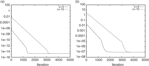
First, we investigate the impact of the initial guess on the convergence of the GD algorithm. We start by considering the following perturbation: Test 1: This represents a strong perturbation in the initial guess. In Figure 1, we plot the convergence history of the objective function and (e⁰)⁽ⁱ⁾ as a function of the iteration number for the complete assimilation. The results for the incomplete assimilation are presented in Figure 2. From both the figures it is observed that the GD algorithm remains convergent.

Figure 1. Convergence history of the objective function (a) and (e⁰)⁽ⁱ⁾ (b) in the complete assimilation.

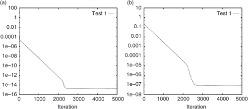
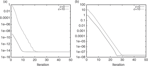
Figure 2. Convergence history of the objective function (a) and (e⁰)⁽ⁱ⁾ (b) in the incomplete assimilation.

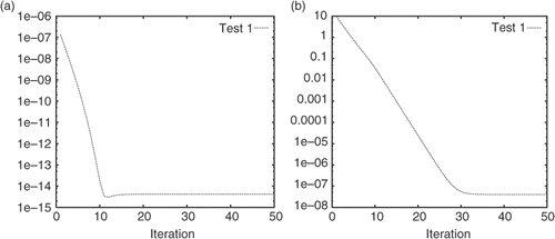
In order to confirm that the presence of perturbation or noise in the initial condition has limited influences on the minimization algorithm, we now consider a very different initial guess; that is we take (u⁰)⁽⁰⁾ to be constant vector c with c = 0 or 10, which has nothing to compare with the exact initial condition sin(πx). We repeat the same computation as in Figures 1 and 2 except for the initial guess. The results are given in Figures 3 and 4. Comparing these results with the ones shown in Figures 1 and 2, we can state that the type and amplitude of the perturbation have no significant effects on the convergence of the minimization algorithm, since in any case the iterative algorithm converges at the same rate.

Figure 3. Same as in Figure 1 except for the initial guess.

Figure 4. Same as in Figure 2 except for the initial guess.

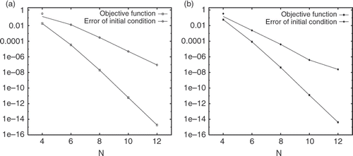
Figure 5. The convergence rate of the objective function and error of initial condition at the optimal state in the complete case (a) and incomplete case (b).

It is worthwhile noting that the convergence of the GD minimization algorithm in the incomplete assimilation is much faster than that in the complete assimilation. One explanation of this phenomena is that the complete assimilation involves much more observation data to be assimilated.

Test 2: The initial guess is set to 0. We investigate the convergence property of the objective function and the optimal initial condition with respect to the polynomial degree N used in the space approximation. In Figure 5, we plot, in a semi-logarithmic scale, the objective function and the error of initial conditions with respect to N. The result for the complete assimilation is given in the left figure, and the incomplete case in the right figure. We observe that both converge exponentially which is a typical behaviour for spectral methods. This means that the spectral methods enable us to achieve highly accurate solution with few grid points. This is of particular importance because practical applications of data assimilation demand for consideration of high-dimensional problems.

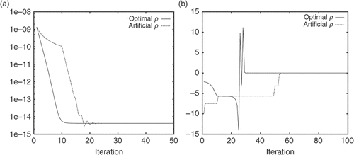
Test 3: Comparison on determinations of the step size. We aim at demonstrating the advantage of our optimal choice method proposed in Section 4.2. To this end, we carry out a numerical test by using different methods for the determination of the step size. The initial guess is again set to zero. In Figure 6, we compare the convergence speeds of the GD algorithm by using our optimal choice method, comparing to the method used in, e.g. 22,25. Figure 6(a) gives the convergence history of the objective function, while the Figure 6(b) plots the obtained step sizes as a function of the iteration. It is clear that our optimal choice method for ρ leads to a faster convergence as compared to the method in 22,25. Moreover, we have found that for the old method in average four values of ρ have to be tested to reach a decreasing objective function.

Figure 6. Comparison of different methods for determination of the step size (a) convergence history of the objective function (b) obtained step sizes.

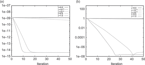
Test 4: Sensitivity to the regularization parameter γ. The purpose of this test is to check the role of the regularization parameter γ used in the incomplete assimilation. The GD algorithm starts again with the initial guess 0. In Figure 7 we present the convergence behaviour of the GD algorithm for several different values of γ. It is observed that the GD algorithm has better convergence property for γ of unit order. The convergence slows down if γ is decreased. Finally, we found that the GD algorithm fails to converge if γ is set to 0.

Figure 7. Impact of γ on the convergence property of the minimization algorithm.

6. Conclusions

In summary, we have presented two efficient methods for discrete adjoint assimilations. The two methods are designed for the initial condition optimization, for complete and incomplete assimilations. The main ingredient of the methods includes:

•	The Crank–Nicolson scheme and the spectral method are applied to establish the fully discrete numerical system. Since the spectral method produces exponential convergence for smooth parameters, the use of this method allows for the application of our parameter optimization to more practical problems.
•	Efficient methods to solve the parameter optimization problems, together with the fast evaluation techniques for the gradient of the objective functions, and an optimal determination of the step sizes.
•	A regularization method for the minimization problem in case of incomplete assimilation, together with a numerical justification of the regularization parameter;
•	A series of numerical tests are carried out to demonstrate the efficiency of the proposed methods.

Although the methods are designed for the optimization of the initial condition, we hope that they are generalizable for the minimization problems of other parameters, such as boundary conditions and/or equation coefficients, etc.

Acknowledgements

This work was partially supported by National NSF of China under Grant 10531080, the Excellent Young Teachers Program by the Ministry of Education of China and 973 High Performance Scientific Computation Research Program 2005CB321703.

References

- W.J. Martin, Initial condition sensitivity analysis of a mesoscale forecast using very large ensembles, in 20th Conference on Weather Analysis and Forecasting/16th Conference on Numerical Weather Prediction, Seattle, WA, 2004..
- Alves, O, Balmaseda, MA, Anderson, D, and Stockdale, T, 2004. Sensitivity of dynamical seasonal forecasts to ocean initial conditions, Q. J. Roy. Meteor. Soc. 130 (597) (2004), pp. 647–667.
- Kirk, DE, 1970. Optimal Control Theory. Englewood Cliffs, NJ: Prentice-Hall; 1970.
- Kirk, DE, 2004. Optimal Control Theory: An Introduction. New York: Courier Dover Publications; 2004.
- Griebel, M, Dornseifer, T, and Neunhoeffer, T, 1998. Numerical Simulation in Fluid Dynamics: A Practical Introduction. Philadelphia, PA: Society for Industrial and Applied Mathematics; 1998.
- Zou, X, Navon, I-M, and Le Dimet, F-X, 1992. An optimal nudging data assimilation scheme using parameter estimation, Q. J. Roy. Meteor. Soc. 118 (508) (1992), pp. 1163–1186.
- Stauffer, DR, and Bao, JW, 1993. Optimal determination of nudging coefficients using the adjoint equations, Tellus A 45 (5) (1993), p. 358.
- Panchang, VG, and OBrien, JJ, 1990. On the determination of hydraulic model parameters using the strong constraint formulation, Model. Marine Syst. 1 (1990), pp. 5–18.
- Smedstad, OM, and O'Brien, JJ, 1991. Variational data assimilation and parameter estimation in an equatorial Pacific Ocean model, Prog. Oceanogr. 26 (1991), pp. 179–241.
- Eknes, M, and Evensen, G, 1997. Parameter estimation solving a weak constraint variational formulation for an Ekman model, J. Geophys. Res. 102 (12) (1997), pp. 479–491.
- Yu, L, and O'Brien, JJ, 1991. Variational estimation of the wind stress drag coefficient and the oceanic eddy viscosity profile, J. Phys. Oceanogr. 21 (5) (1991), pp. 709–719.
- Navon, IM, 1998. Practical and theoretical aspects of adjoint parameter estimation and identifiability in meteorology and oceanography, Dyn. Atmos. Oceans 27 (1–4) (1998), pp. 55–79.
- Le Dimet, FX, and Talagrand, O, 1986. Variational algorithms for analysis and assimilation of meteorological observations: Theoretical aspects, Tellus. Series A, Dyn. Meteorol. Oceanogr. 38 (2) (1986), pp. 97–110.
- Lewis, JM, and Derber, JC, 1985. The use of adjoint equations to solve a variational adjustment problem with advective constraints, Tellus. Series A, Dyn. Meteorol. Oceanogr. 37 (4) (1985), pp. 309–322.
- Ortega, JM, and Rheinboldt, WC, 2000. Iterative Solution of Nonlinear Equations in Several Variables. USA: Society for Industrial and Applied Mathematics Philadelphia; 2000.
- Zitong, C, Tongli, S, Yihui, D, and Linping, S, 1998. Data assimilation system for mesoscale models. Part I: Layout o fan adjoint model, J. Nanjing Institute of Meteorology 21 (2) (1998), pp. 165–172.
- Parter, SV, and Rothman, EE, 1995. Preconditioning Legendre spectral collocation approximations to elliptic problems, SIAM J. Numer. Anal. 32 (1995), pp. 333–385.
- Quarteroni, A, and Valli, A, 1994. Numerical Approximation of Partial Differential Equations. Berlin: Springer; 1994.
- Sirkes, Z, and Tziperman, E, 1997. Finite difference of adjoint or adjoint of finite difference?, Mon. Weather Rev. 125 (12) (1997), pp. 3373–3378.
- Bernardi, C, Maday, Y, and Rapetti, F, 2004. Discrétisations Variationnelles de Problèmes aux Limites Elliptiques. Berlin: Springer; 2004.
- Canuto, C, Hussaini, MY, Quarteroni, A, and Zang, TA, 1988. Spectral Methods in Fluid Dynamics. Berlin: Springer; 1988.
- Huang, S, Wei, H, and Rongsheng, W, 2004. Theoretical analyses and numerical experiments of variational assimilation for one-dimensional ocean temperature model with techniques in inverse problems, Sci. China Ser. D: Earth Sci. 47 (7) (2004), pp. 630–638.
- Zou, X, Navon, IM, and Le Dimet, F-X, 1992. Incomplete observations and control of gravity waves in variational data assimilation, Tellus A 44A (1992), pp. 273–296.
- Sixun Huang, Jie Xiang, Huadong Du, and Xiaoqun Cao. Inverse problems in atmospheric science and their application. J. Phys. Conf. Ser. 12 (2005), pp. 45–57..
- Kalnay, E, Park, SK, Pu, ZX, and Gao, J, 2000. Application of the quasi-inverse method to data assimilation, Mon. Weather Rev. 128 (3) (2000), pp. 864–875.