A numerical method for solving the inverse heat conduction problem without initial value

Abstract

We consider the inverse heat conduction problem for the one-dimensional heat equation, where we are requested to determine a boundary value at one end of a spatial interval over a time interval and an initial value by means of Cauchy data at another end. By the existing theory we can prove the uniqueness in determining both a boundary value and an initial value, and our method does not require any initial value. We test our numerical method and show stable numerical reconstruction.

Keywords:

• inverse heat conduction problem
• truncated Fourier series
• numerical reconstruction

AMS Subject Classifications::

• 35R25
• 35R30
• 35K05

1. Introduction

The inverse heat conduction problem arises in most thermal manufacturing processes of solids and has recently attracted much attention. In this inverse problem, for the heat equation, one is requested to reconstruct a heat flux or boundary temperature on an inaccessible subboundary. The typical case is the determination of the heat flux on an inaccessible subboundary through measurements on an accessible subboundary. In the real applications, only discrete data with noises at finite points are available. This problem is known to be extremely ill-posed (e.g. 1), that is, small perturbations in data may cause dramatically large errors in the solution. Therefore for stable numerical reconstruction, we need stabilization or regularization techniques. For general treatment of such techniques, see for example 2,3.

As for numerical methods for the inverse heat conduction problem, there are many works and we refer, for example, to 1,20–22 and the references therein. In most of the existing works, initial data are assumed to be given, although one knows the uniqueness in determining both a boundary value and an initial value by Cauchy data (e.g. 18,19). In particular, in 17, Takeuchi develops a numerical method for the inverse heat conduction problem without the information of initial values and our method is more direct.

In many practical situations such as an on-line testing, we cannot know the initial condition because we have to estimate the problem for the heat process which was already started.

The main purpose of this article is to propose a numerical method which does not need initial data for the reconstruction of boundary values and is stable against the intrinsic instability of the inverse heat conduction problem. Our method can be implemented for heat equations with variable coefficients in general spatial dimensions, but here we will exclusively discuss the one-dimensional heat equation with constant coefficients for demonstrating the essence of our method. As for a basic idea for the numerical scheme in such a general case, see the Appendix. As for other kinds of ill-posed problems for the heat equation, we refer to 20–22.

2. Formulation of the problem and algorithm

We consider the one-dimensional heat equation: (1) Here α > 0 is a given constant. For (2.1), we discuss the following.

Inverse heat conduction problem: Determine (2) and (3) from (4) and (5)

Then we can prove the uniqueness in the heat conduction problem: g(t), h(t), 0 ≤ t ≤ T uniquely determine f(t), 0 ≤ t ≤ T and u₀(x), 0 ≤ x ≤ 1 (e.g. Theorem 3.3.10 (p. 63) in 18) and Section 1 of Chapter IV in 19). As for the related theoretical results, see 23,24 for example.

Let 0 < t₁ < ··· < t_M be given. Our target is to reconstruct the value of f(t) and u₀(x) from discrete noisy values of g(t_j) and h(t_j), j = 1, 2, …, M.

Our primary interest is the reconstruction of f(t), and the boundary value is often a more serious influence for controlling the heat process from the practical point of view.

Set and Then we can represent a solution u to (2.1) by 25–27: where and

The terms and cause the instability for the computation. Hence, we will try to avoid the integration by solving the following forward problem.

Define (6) and Then we have (7) Here v(ℓ, t) can be taken by solving the forward problem of (2.6), so ω(ℓ, t) is given.

The solution to (2.7) can be represented by where and Suppose that {0 = t₀ < t₁ < ··· < t_M = T} is a uniform grid of the time interval [0, T]. Then at time t_j, we have the following approximation equation:

THEOREM 2.1

Define Then satisfies (8) Here

Proof

In terms of a change of independent variables: defined by and , we can reduce the heat equation (2.1) to , , , so that we can assume that ℓ = 1 and α = 1 without loss of generality. Here we write x and t in place of and . Since and it is easy to see that

Define and We know that 25, Lemmas 6.2.3 and 6.2.5, pp. 60–61]. Also, since we can prove that similarly to 27, Theorem 4.1, p. 90], for t > 0 we have and Furthermore, when t > t_i, (e.g. 25, p. 60]). According to the result of Lemma 6.2.1 on p. 60 in 25, we know that for t > 0. Moreover, since we have This completes the proof of the theorem.

This theorem can be proved in general dimensions, but here we use a more direct way for the proof in one-dimensional case.

Let for j ≥ i and for j < i. Then We define an M × (M + N + 1) matrix P by where we set and Setting we have By solving this linear equations, we can obtain the values f(t_i), 1 ≤ i ≤ M. However, since P is an M × (N + M + 1) matrix, it is under-determining. For specifying a solution more stably, we introduce an additional constraint for a solution f(t_i), i = 1, …, M. That is, assume that M = 2M₀ and f(t_2i) = f(t_2i−1), i = 1, …, M₀. Set an M × (M₀ + N + 1) matrix: where we define an M × M₀ matrix and an (M₀ + N + 1)-vector by and Then and it is an over-determined linear system with the extra constraints f(t_2i) = f(t_2i−1), i = 1, …, M₀. Using the constraint, we can limit the set of solutions and expect better numerical performances, which is verified by numerical tests in Section 3.

3. Numerical results

In this section, we will give some numerical examples to test the algorithm given in the previous section. First, we will give an example where the exact solution is known. We add some random noises to the measured data and use these data to test our algorithm.

We set and 0 = t₀ < t₁ < ··· < t₂₀₀ = 2 is a uniform grid of [0, 2], i.e. . , are given and we want to calculate the value of and u(0, t). We will try different values of K.

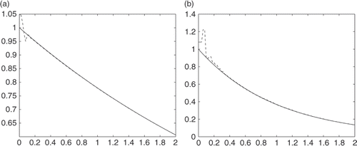
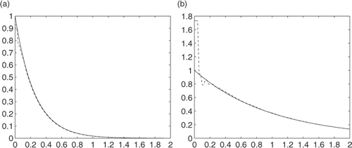
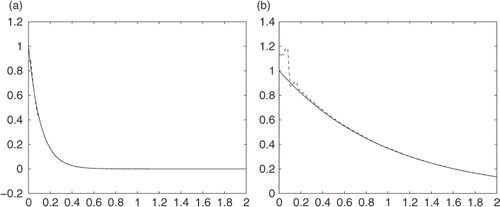
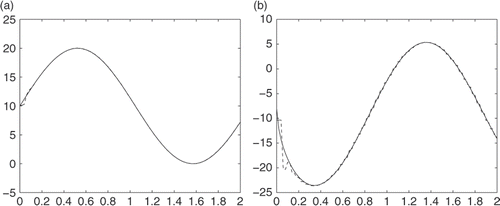
Figure 1 shows the numerical results where the measurement data has no noise. Henceforth, the solid lines in the figures indicate the exact values and dashed lines indicate the numerical results.

Figure 1. Schematic representation of K = 0.5, without noise: (a) u(0, t) and (b) .

FromFigure 1, we can see that for u(0, t) the calculated value is quite close to the exact value and for , the result is good when t is large enough. For small t, the numerical performances are bad because we do not know the initial data.

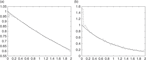
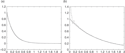
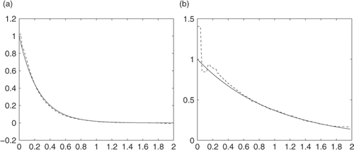
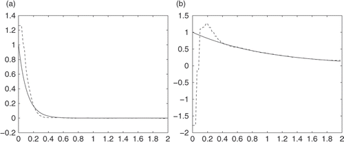
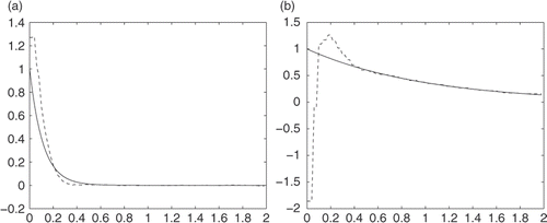
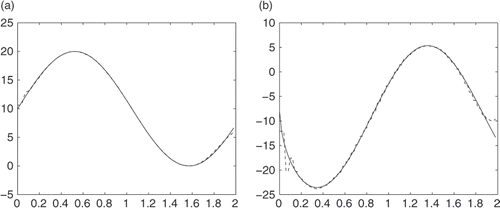
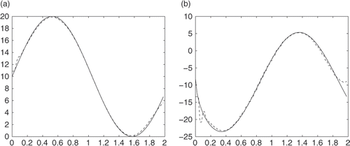
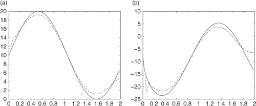
Next we will give some random noises to the measurement data. Also, since the measurement data with random noise are oscillating, we will use some skills to smooth the measurement data first and then apply our algorithm. Here we use the numerical differentiation method to smoothen the measurement data 28. Figures 2–4 indicate the numerical results for u(0, t) and in various cases of noise levels.

Figure 2. Schematic representation of K = 0.5, with 0.5% random noise: (a) u(0, t) and (b) .

Figure 3. Schematic representation of K = 0.5, with 1% random noise: (a) u(0, t) and (b) .

Figure 4. Schematic representation of K = 0.5, with 3% random noise: (a) u(0, t) and (b) .

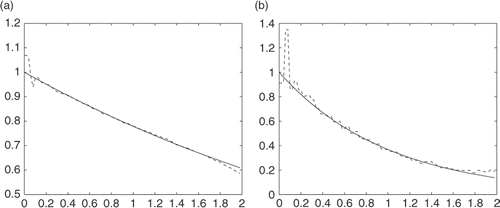
Next we will show the numerical results with different values of K (Figures 5–12).

Figure 5. Graph of K = 2, without noise: (a) u(0, t) and (b) .

Figure 6. Graph of K = 2, with 0.5% random noise: (a) u(0, t) and (b) .

Figure 7. Graph of K = 2, with 1% random noise: (a) u(0, t) and (b) .

Figure 8. Graph of K = 2, with 3% random noise: (a) u(0, t) and (b) .

Figure 9. Graph of K = 3, without noise: (a) u(0, t) and (b) .

Figure 10. Graph of K = 3, with 0.5% random noise: (a) u(0, t) and (b) .

Figure 11. Graph of K = 3, with 1% random noise: (a) u(0, t) and (b) .

Figure 12. Graph of K = 3, with 3% random noise: (a) u(0, t) and (b) .

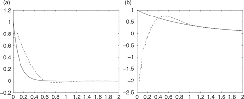
From these numerical tests, we can see that errors are large near t = 0, but better when t is large enough; the results for u(0, t) are quite good, and results for are acceptable.

We will also show the L²-norms of the differences between the exact solution and the reconstructed solutions in the time interval (0.2, 2).

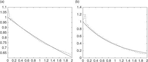
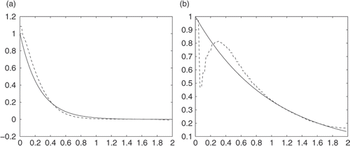
In the next example, we will show the case in which the exact solution is not given. We will use the finite difference method to solve the forward problem and take data at one side of the boundary. Taking some random noises and applying our method, we can obtain the reconstructed values at another side of the boundary. We compare these results with the data given by the finite difference method (Table 1).

Table 1. Absolute errors with different noise level and K.

K	Noise level	Errors for u(0, t)	Errors for
0.5	0	0.00095	0.0090
0.5	0.5%	0.0058	0.0270
0.5	1%	0.0080	0.0282
0.5	3%	0.0127	0.0296
2	0	0.0035	0.0079
2	0.5%	0.0070	0.0158
2	1%	0.0086	0.0316
2	3%	0.0348	0.0595
3	0	0.0011	0.0091
3	0.5%	0.0150	0.1132
3	1%	0.0157	0.1137
3	3%	0.1342	0.2568

The solution itself satisfies the following equations: (9) The numerical results are given in Figures 13–16.

Figure 13. Graph of (a) u(0, t) and (b) , without random noise.

Figure 14. Graph of (a) u(0, t) and (b) , with 0.5% random noise.

Figure 15. Graph of (a) u(0, t) and (b) , with 1% random noise.

Figure 16. Graph of (a) u(0, t) and (b) , with 3% random noise.

Table 2 gives the L² norm of the errors in the time interval (0.2, 2).

Table 2. Absolute errors with different noise level.

Noise level	Errors for u(0, t)	Errors for
0	0.0426	0.4233
0.5%	0.1604	0.8297
1%	0.2675	1.0645
3%	0.9866	2.4189

Acknowledgements

The authors thank the anonymous referees for valuable comments.

Appendix

Let Ω ⊂ R^d be a bounded domain with smooth boundary ∂Ω and, , ν = ν(x) = (ν₁, …, ν_d) denotes the unit outward normal vector to ∂Ω at x, and Γ ⊂ ∂Ω be a subboundary. We consider where a and b are sufficiently smooth and a > 0 on . We set We consider the following problem.

Inverse heat conduction problem: Determine and from and Similarly to (2.7), we can assume that g(x, t) = 0, x ∈ Γ, 0 < t < T. We consider the set of the eigenvalues of −A with the boundary condition on ∂Ω and number them according to the multiplicities: (10) That is, if for an eigenvalue λ_i, there exist ℓ linearly independent eigenfunctions v₁, …, v_ℓ: −Av_j = λ_iv_j in Ω and on ∂Ω for j = 1, …, ℓ, then λ_i appear ℓ-times in the sequence (1).

By Itô 26 and g = 0 on Γ, there exists the fundamental solution G(t, x, y), x, y ∈ Ω, t > 0 such that we can represent u = u(x, t) by (11) with some functions B_n(x), provided that u satisfies some conditions on the smoothness. In order to numerically reconstruct , x ∈ ∂Ω ∖ Γ, 0 < t < T, we introduce a suitable system {ψ_k}_1≤k≤N1 of linearly independent functions on (∂Ω ∖ Γ) × (0, T) and we approximate f by a finite sum and replace by with suitable natural number N₂. Then, choosing x_ℓ ∈ Γ, ℓ = 1, …, L₁, t_m ∈ (0, T), m = 1, …, M₁, on the basis of (2), we search an approximation satisfying (12) Here we set (13) Considering (3) as a linear system and solving with respect to a₁, …, a_N1, B_n(x_ℓ), ℓ = 1, …, L₁, n = 1, …, N₂, we can obtain an approximation for on (∂Ω × Γ) × (0, T). In order to calculate the coefficient matrix of the linear system (3), we have to obtain N₂ eigenvalues λ₁, …, λ_N2 and G_k(x_ℓ, t_m). For λ_k, we can use a suitable numerical method for finding eigenvalues. Moreover, under suitable conditions on ψ_k, since we can verify (e.g. 26) that G_k satisfies We can calculate G_k(x_ℓ, t_m) by numerically solving this initial value–boundary value problem. Due to the ill-posedness of the inverse heat conduction problem, we have to choose appropriate N₁, N₂ and apply a suitable regularization in stably solving the linear system (3), but here we will not discuss in detail. We note that in the one-dimensional case in Section 2, ∂Ω ∖ Γ consists of one point x = 0, and that we choose

References

- Alifanov, OM, 1994. Inverse Heat Transfer Problems. Berlin: Springer-Verlag; 1994.
- Engl, HW, Hanke, M, and Neubauer, A, 1996. Regularization of Inverse Problems. Dordrecht: Kluwer; 1996.
- Groetsch, CW, 1984. The Theory of Tikhonov Regularization for Fredholm Equations of the First Kind. Boston: Pitman; 1984.
- Eldén, L, 1995. Numerical solution of the sideways heat equation by difference approximation in time, Inverse Probl. 11 (1995), pp. 913–923.
- Beck, JV, Blackwell, B, and Clair, CRS, 1985. Inverse Heat Conduction. Hoboken, NJ: John Wiley & Sons; 1985.
- Fu, C, Xiong, X, and Li, H, 2005. Fourier regularization for determining surface heat flux from interior observation based on a sideways parabolic equation, Numer. Math. J. Chin. Univ. (English Ser.) 14 (2005), pp. 208–216.
- Lattès, R, and Lions, J-L, 1969. The Method of Quasi-reversibility, Applications to Partial Differential Equations. New York: American Elsevier Publishing Co., Inc.; 1969.
- Hào, DN, 1998. Methods for Inverse Heat Conduction Problem. Peter Lang, Frankfurt am Main; 1998.
- Hào, DN, and Reinhardt, H-J, 1996. Stable numerical solution to linear inverse heat conduction problems by the conjugate gradient method, J. Inverse Ill-Posed Probl. 3 (1996), pp. 447–467.
- Hào, DN, Reinhardt, H-J, and Schneider, A, 2001. Numerical solution to a sideways parabolic equation, Int. J. Numer. Methods Eng. 50 (2001), pp. 1253–1267.
- Hon, YC, and Wei, T, 2005. The method of fundamental solution for solving multidimensional inverse heat conduction problems, CMES Comput. Model. Eng. Sci. 7 (2005), pp. 119–132.
- Matsuura, T, Saitoh, S, and Trong, DD, 2005. Approximate and analytical inversion formulas in heat conduction on multidimensional spaces, J. Inverse Ill-Posed Probl. 13 (2005), pp. 479–493.
- Murio, DA, 1993. The Mollification Method and the Numerical Solution of Ill-posed Problems. New York: John Wiley; 1993.
- Regińska, T, and Eldén, L, 1997. Solving the sideways heat equation by a wavelet-Galerkin method, Inverse Probl. 13 (1997), pp. 1093–1106.
- Shidfar, A, and Pourgholi, R, 2006. Numerical approximation of solution of an inverse heat conduction problem based on Legendre polynomials, Appl. Math. Comput. 175 (2006), pp. 1366–1374.
- Stolz, G.Tr., 1960. Numerical solution to an inverse problem of heat condition for simple shapes, ASME J. Heat Transfer 82 (1960), pp. 20–26.
- Takeuchi, T, , An inverse numerical method by reproducing kernel Hilbert spaces and its applications to linear inverse problem, Doctoral thesis, Graduate School of Mathematical Sciences, The University of Tokyo, 2007..
- Isakov, V, 2006. Inverse Problems for Partial Differential Equations. Berlin: Springer-Verlag; 2006.
- Lavrent'ev, MM, Romanov, VG, and Shishat·skiĭ, SP, 1986. Ill-posed Problems of Mathematical Physics and Analysis. Providence, RI: American Mathematical Society; 1986.
- Klibanov, MV, 2006. Estimates of initial conditions of parabolic equations and inequalities via lateral Cauchy data, Inverse Probl. 22 (2006), pp. 495–514.
- Li, J, Yamamoto, M, and Zou, J, 2009. Conditional stability and numerical reconstruction of initial temperature, Commun. Pure Appl. Anal. 8 (2009), pp. 361–382.
- Wei, T, and Yamamoto, M, 2009. Reconstruction of a moving boundary from Cauchy data in one dimensional heat equation, Inverse Probl. Sci. Eng. 17 (4) (2009), pp. 551–567.
- Klibanov, MV, and Timonov, AA, 2004. Carleman Estimates for Coefficient Inverse Problems and Numerical Applications. Utrecht: VSP; 2004.
- Vessella, S, 2008. Quantitative estimates of unique continuation for parabolic equations, determination of unknown time-varying boundaries and optimal stability estmates, Inverse Probl. 24 (2008), p. 023001 (81 pp).
- Cannon, JR, 1984. The One-dimensional Heat Equation. California: Addison-Wesley; 1984.
- Itô, S, 1992. Diffusion Equations. Providence, RI: American Mathematical Society; 1992.
- Widder, DV, 1975. The Heat Equation. New York: Academic Press; 1975.
- Wang, YB, Jia, XZ, and Cheng, J, 2002. A numerical differentiation method and its application to reconstruction of discontinuity, Inverse Probl. 18 (2002), pp. 1461–1476.