Tomography reconstruction by entropy maximization with smoothing filtering

Abstract

The maximum entropy method (MEM) is a consistent way to treat the problem of tomography reconstruction where an image should be selected from a set of images that fit the measurement data. In this article, MEM is applied to image reconstruction from projections using an entropy formula modified by adding filter terms in order to eliminate the local noise. Numerical experiments were performed showing good results with local mean-square filter terms. The projection error can be used to estimate the weight of the filter term, providing a practical procedure to get improved solutions with limited sets of projections.

Keywords:

• maximum entropy
• tomography
• image processing
• image reconstruction
• radiography

1. Introduction

Computerized tomography (CT) is a method of constructing an image of the inner structure of an object taking a finite set of measurements of the radiation attenuated by the object at different projection angles as input data. CT has many well-known applications in a variety of problems including medical imaging diagnostics and non-destructive testing. Formally, the mathematical problem is to find the solution of the Radon anti-transformation of a spatial scalar field 1, which falls into the domain of inverse problems.

In the applications of industrial tomography for the quality control of manufacturing process, usually only a small number of projections is available to avoid delays, and thus the problem is underdetermined. In turn, a priori data is often available in these cases, which can be used to balance the information process 2. The maximum entropy method (MEM) was proposed to solve CT problems by several authors 3–6, being an alternative to other methodologies as the algebraic reconstruction, filtered back projection and convolution back projection, along with many variants of these techniques 1,7. The Radon anti-transformation by MEM is generally solved by means of an iterative optimization algorithm, showing flexibility to handle noisy data and incomplete projections more easily than other methods. An important advantage of MEM is the flexibility to incorporate prior information available in addition to that contained in the projection data. Particularly in industrial tomography, this kind of conformation is usually available from the design or manufacturing processes (e.g. internal shapes, porosity and smoothness). In this article, we propose to apply MEM for CT incorporating additional terms to the entropy to filter the noise in the final image.

Previously, there were several proposals to use a priori information in CT reconstruction methods 8–11. The MEM principle is used in maximum a posteriori (MAP) algorithms 7,6, in the form of the penalized maximum log-likelihood (PML) with entropy (MEM) and Gibbs priors 8,10, or in other case with penalized least squares (PLS) with priors function like Shannon entropy among others 5,6. In PML, the Poisson nature of noise in the data explicitly enters in the algorithm whereas it is indirect in PLS 5,6,8,10. In this study, tomographic reconstructions follows the PLS with entropy priors. The novelty introduced here is the addition of a smoothing filter as Gibbs priors in cases where the homogeneity of the image components is known. The proposal approach is tested with very few projections distributed uniformly over the full 180 degrees. Examples of reconstructions from the ideal projections or projections with random uniform noise are analysed.

2. Tomographic reconstruction by modified MEM

MEM 11 is a general mathematical procedure for solving inverse problems where the available data is insufficient to determine the solution. MEM provides an adequate way of selecting a single image from the many images that are consistent with the incomplete input data, by determining the solution that introduces the minimum information extrinsic to the available data.

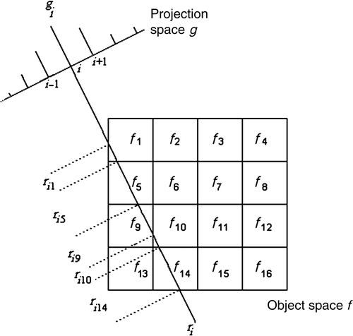
Let f denote the image to be reconstructed, represented by an n-dimensional column vector. Let R be an m × n projection matrix, whose r_ij element denotes the coefficient of the contribution of the j-pixel to the i-ray (Figure 1). Then, the discrete Radon transform of f is defined as (1) where g is an m-dimensional projection vector (i.e. m rays are projected through f). In general, m < n. The CT problem consists of finding f given R and g.

Figure 1. Image space f and the ith ray crossing the object.

The MEM reconstruction consists of determining a suitable solution of f whose Shannon entropy (2) is maximum among all solutions consistent with (1). Here it is proposed to extend the MEM requirements to also minimize a smoothness energy U(f), i.e. (3)

In this way, MEM can be applied to situations where it is previously known that f represents internally smooth objects whose characteristic length is much larger than a pixel side. This prior information can be modelled by means of interactions among neighbour pixels. Two possible quadratic models based on a 3 × 3 neighbourhood interaction are: (4) (5) where ⟨N_j⟩ is the average intensity of the 3 × 3 cluster N_j and E₁(N_j) and E₂(N_j) are suitable indicators of the local ‘noise’, both vanishing in the extreme case of homogeneous clusters.

The smoothness energy U(f) is defined as: (6) where β is a calibration constant, E is given by (4) or (5), and the summation in (6) is performed over all the clusters of the image f. U(f) can also be written in matrix form as: (7) where M is an n × n matrix whose elements m_jv are defined by the form of the function E(N_j), as defined by (4) or (5), respectively. The matrix M can also be thought as a regularization operator 12–15.

Thus, the cell m_jv of the matrix M when (4) is used is defined as (8) where N_j are the nearest 3 × 3 neighbours of the pixel j, and |N_j| is the cardinality of this subset.

When Equation (5) is used, the cell m_jv of the matrix M is defined as (9) where N_j and N_v are the nearest 3 × 3 neighbours of the pixel j or v, respectively.

Combining (3) and (7), the optimization problem reads (10) where in log f, the logarithm is taken for each component of the vector f.

The corresponding Lagrangian L(f, λ) is as follows: (11)

Making zero the derivatives of L(f, λ) leads to the following system S(f): (12)

The non-linear system S(f) = 0 needs to be solved numerically applying some root finding scheme. In this study, the classic Newton method was applied 16. The method is iterative starting from an initial guess f₀, and producing successive approximations f_n by adding a correction factor δ_f, i.e. (13)

The unknown variables of the problem are δ_f (n-dimensional vector) and δ_λ (m-dimensional vector of Lagrange multipliers), the combination of which will be called as vector δ and should satisfy (14) where J_fn is the (n + m)² dimensional Jacobian matrix of the system S(f) evaluated at f_n: (15)

Combining Equations (12), (14) and (15), the following Newton system is obtained: (16)

To fulfil the non-negative condition of f, negative values of f components are reset to small positive values after each iteration.

3. Results

The proposed algorithm was implemented on a 2D reconstruction problem from eight projections corresponding to 0, 30, 60, 75, 90, 105, 120 and 150 degrees, 20 parallel rays each. Figures 2 and 3 show the reconstructed 20 × 20 pixel images obtained for various values of β. In Figure 2, the M matrix was defined using the interaction function E₁, whereas in Figure 3 the function U was constructed using E₂.

Figure 2. Reconstructions with different parameters of β and the matrix M calculated with Equation (4). Notes: (a) β = 0, (b) β = 50, (c) β = 10², (d) β = 10³, (e) β = 10⁴ and (f) β = 10⁶.

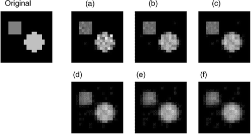
Figure 3. Reconstruction with different parameters of β and the M matrix calculated with Equation (5). Notes: (a) β = 0, (b) β = 50, (c) β = 10², (d) β = 10³, (e) β = 10⁴ and (f) β = 10⁶.

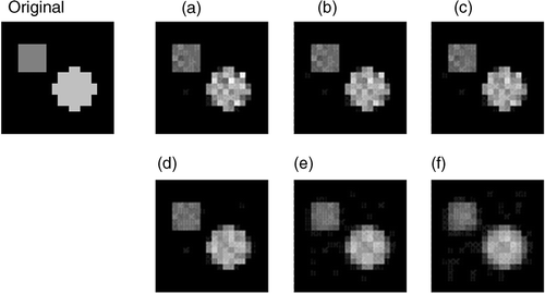
When β is zero, the algorithm reduces to the classical MEM method 11. As β increases, a smoothing progression can be observed. The term U increasingly penalizes the difference between neighbouring pixels, thus forcing them to become similar. When β increases beyond a certain large value the borders of the object begin to blur.

In order to estimate the quality of the reconstruction, the pixel-to-pixel error σ is defined as (17) where f ^data and f are n-dimensional vectors of the original and the reconstructed image, respectively (note that σ is an indicator that is only known in simulated cases where the original image is known).

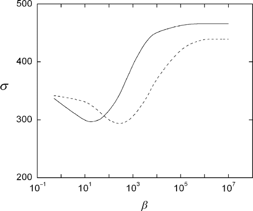
Figure 4 shows the dependence of σ with β. A minimum can be observed, which indicates an optimum β value. Lower values of β lead to image degradation, whereas higher values of β produce blurring. This effect can be clearly seen in Figures 2 and 3.

Figure 4. Pixel-to-pixel error between the reconstructed and the original image, using Equations (4) (solid) and (5) (dashed).

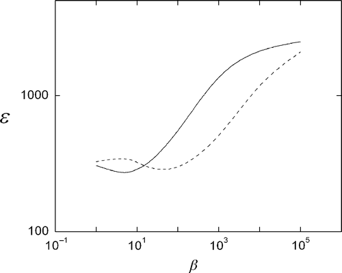
Figure 5 shows the projection error ε: (18) where g^data and g are m-dimensional vectors of the data projections and the reconstructed image projections, respectively. It can be seen that with respect to the projection error ε there is also an optimum value β, which although is slightly different than the one produced with σ (Figure 4), it is more useful since ε can always be calculated, whereas σ is only available in controlled cases where the solution is known.

Figure 5. Error between projections of the reconstruction image and the projection data, using Equations (4) (solid) and (5) (dashed).

Figures 6 and 7 show the reconstruction of a 64 × 64 pixels image with three internal circles, using 16 projections (64 rays per projection). Figures 8 and 9 show the error parameters ε and σ as functions of β. A behaviour similar to Figures 2–5 can be observed, that is, starting with β = 0 successive increases of β improve the reconstruction quality by noise filtering, up to certain β value from which further increments lead to excessive blurring of the internal borders.

Figure 6. Reconstructions with different β using Equation (4). Notes: (a) β = 0, (b) β = 10³, (c) β = 10⁴ and (d) β = 10⁶.

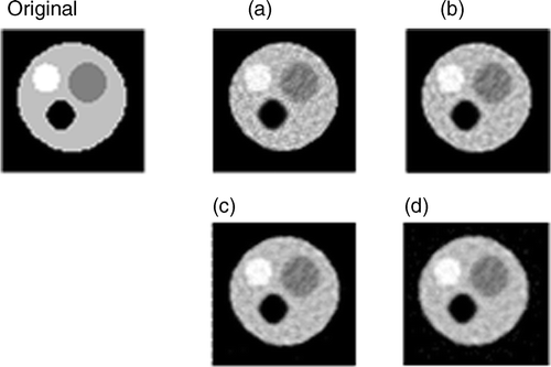
Figure 7. Reconstructions with different β using Equation (4). Notes: (a) β = 0, (b) β = 10³, (c) β = 10⁴, and (d) β = 10⁶.

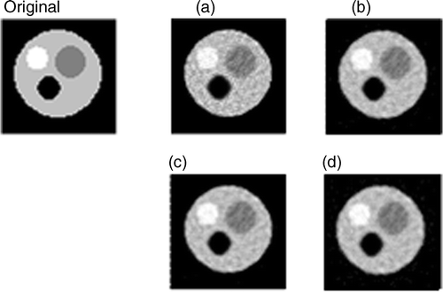
Figure 8. Pixel-to-pixel standard deviation between the reconstructed and the original image, using Equations (4) (solid) and (5) (dashed).

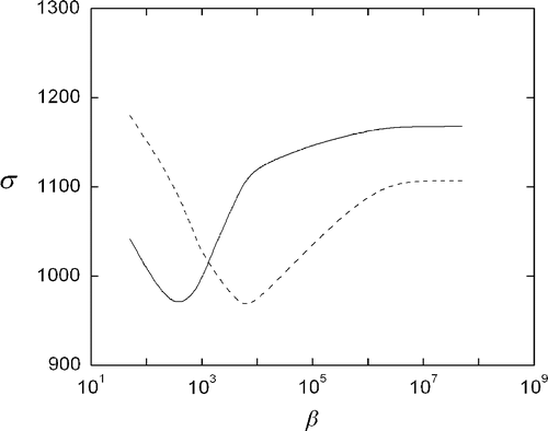
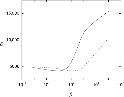
Figure 9. Error between projections of the reconstruction image and the noiseless projection data, using Equations (4) (solid) and (5) (dashed).

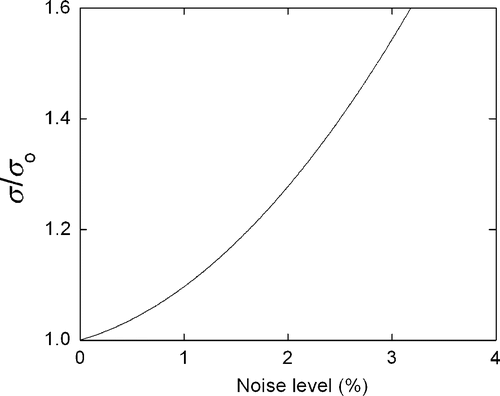
It is interesting to test the performance of the proposed method on noisy data. The case shown in Figure 6 was used as reference, adding artificially random noise to the projection data. Figures 10 and 11 show the dependence of the pixel-to-pixel error σ and projection error ε on β using Equations (4) and (5). It can be seen that the behaviour of σ is similar to Figure 8 (noiseless projections), although the optimum values of β differ. Nevertheless, as in the noiseless case, the minimum of ε can be used to estimate an appropriate value of β. Figures 12 and 13 show the reconstructions obtained by varying β combined with Equations (4) and (5), respectively. The quality of the reconstructions logically decreases as the noise increases. This feature can be appreciated in Figure 14, which shows how the pixel-to-pixel error increases with respect to the noiseless value as the noise level of the projections increases.

Figure 10. Pixel-to pixel error between the reconstructed image and the original image data, using Equations (4) (solid) and (5) (dashed), and projections data with 2% random uniform noise.

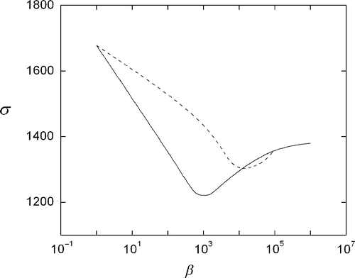
Figure 11. Error between projections of the reconstruction image and the noisy projection data, using Equations (4) (solid) and (5) (dashed).

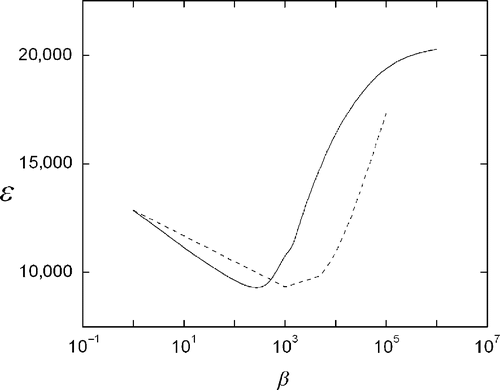
Figure 12. Reconstructions with 2% random-noise projections with Equation (4). Notes: (a) β = 0, (b) β = 10³, (c) β = 10⁴ and (d) β = 10⁵.

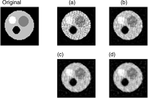
Figure 13. Reconstructions with 2% random-noise projections with Equation (5). Notes: (a) β = 0, (b) β = 10³, (c) β = 10⁴ and (d) β = 10⁵.

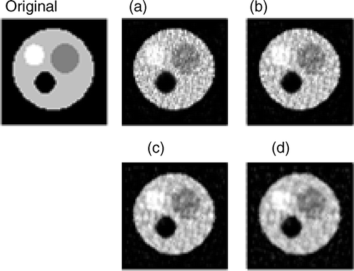
Figure 14. Increment of the pixel-to-pixel error relative to the noiseless value as the noise level of the projections increase.

Table 1 compares the results obtained with different variations of this method, namely, plane MEM without regulation terms (β = 0), and MEM with the optimum β that minimizes the projection error ε. Comparisons were also made by applying a median filter to the solutions. The best results were obtained with MEM regularized with Equation (4). One pass of median filtering reduces the pixel-to-pixel error σ, but increases the projection error ε considerably. Figures 15 and 16 shows the reconstructions corresponding to the cases detailed in Table 1.

Figure 15. Reconstructions with 2% random-noise projections and median filter. Notes: (a–c) planar MEM β = 0 without and with non-linear median filter applied (one pass) and (two pass), (d–e) using Equation (4) and optimum β without and with one pass median filter, (f–g) using Equation (5) and optimum β without and with one pass median filter.

Figure 16. Reconstructions with noiseless projections. Notes: (a–c) planar MEM β = 0 and non-linear median filter applied one pass and two pass, (d–e) using Equation (4) and optimum β without and with one pass median filter, (f–g) using Equation (5) and optimum β without and with one pass median filter.

Table 1. Pixel-to-pixel and projection errors obtained with different reconstructions of Figure 6.

Method	Noiseless projections		Projections with 2% noise
	σ	ε	σ	ε
β = 0	1186	4934	1677	12,864
β = 0 and one median filtering	926	15,199	1154	28,905
β = 0 and two median filtering	903	16,356	1095	32,056
Optimum β (minimum ε) with Equation (4)	917	4213	1267	9027
Optimum β (minimum ε) with Equation (4) and one median filtering	825	10,082	1015	16,858
Optimum β (minimum ε) with Equation (5)	947	4944	1305	10,922
Optimum β (minimum ε) with Equation (5) and two median filtering	869	10,476	1078	18,341

4. Conclusions

The introduction of prior information to the MEM algorithm for computer tomography was presented. A filter term was added to the classical entropy function to improve the a priori known homogeneity of the image. A series of numerical tests were performed comparing variations of this method, showing improvements in the final quality of the image compared to the classical MEM procedure. A heuristic method was proposed to estimate the weight of the filter term based on the minimization of the projection error. The proposed algorithm can be a useful numerical tool, particularly in industrial tomography, where local homogeneity is an often available information from the design and manufacturing processes. Further theoretical studies are required in order to quantify the robustness of the proposed heuristics for the filter coefficient, which will be helpful for applications in the real data set.

References

- Herman, GT, 1980. Image Reconstruction from Projections: The Fundamental of Computerized Tomography. London: Academic Press; 1980.
- Barbuzza, R, Vénere, M, and Clausse, A, 2007. Quality assurance of manufactures by means of intelligent tomographic processing, J. Test. Eval. 35 (2007), pp. 59–65.
- Dusaussoy, NJ, and Abdou, IE, 1991. The extended MENT algorithm: A maximum entropy type algorithm using prior knowledge for computerized tomography, IEEE Trans. Signal Process. 39 (1991), pp. 1164–1180.
- Minerbo, G, 1979. MENT: A maximum entropy algorithm for reconstruction a source from projection data, Comput. Graphics Image Process. 10 (1979), pp. 48–68.
- Mohammad-Djafari, A, Giovannelli, J, Demoment, G, and Idier, J, 2002. Regularization, maximum entropy and probabilistic methods in mass spectrometry data processing problems, Int. J. Mass spectrom. 215 (2002), pp. 175–193.
- Nguyen, M, and Mohammad-Djafari, A, 1994. Bayesian approach with the maximum entropy principle in image reconstruction from microwave scattered field data, IEEE Trans. Med. Imaging 13 (1994), pp. 254–262.
- Herman, GT, and Kuba, A, 1999. Discrete Tomography, Foundations, Algorithms and Applications. Boston: Birkhäuser; 1999.
- Bouman, C, and Sauer, K, 1993. A generalized gaussian image model for edge-preserving MAP estimation, IEEE Trans. Image Process. 2 (1993), pp. 296–310.
- Frese, T, Bouman, A, and Sauer, K, 2002. Adaptive wavelet graph model for Bayesian tomographic reconstructions, IEEE Trans. Image Process. 11 (2002), pp. 756–770.
- Ghosh Roy, DN, Wilton, K, Cook, TA, Chakrabarti, S, Qi, J, and Gullberg, GT, 2004. Tomographic Reconstructions using MAP Algorithms: Application to the SPIDR Mission. Lawrence Berkeley National Laboratory.; 2004, Paper LBNL-54934.
- Jaynes, ET, 1957. Information theory and statistical mechanics, Phys. Rev. 106 (1957), pp. 620–630.
- Bovik, AC, 2005. Handbook of Image and Video Processing. New York: Elsevier Academic Press; 2005.
- Cidade, G, Anteneodo, C, Roberty, N, and Silva Neto, A, 2000. A generalized approach for atomic force microscopy image restoration with Bregman distances as Tikhonov regularization terms, Inverse Probl. Eng. 8 (2000), pp. 457–472.
- Katsaggelos, AK, and Galatsanos, N, 1998. Signal Recovery Techniques for Image and Video Compression and Transmission. New York, LLC: Springer-Verlag; 1998.
- Katsaggelos, AK, Kohonen, T, Schroeder, MR, and Huang, TS, 1991. Digital Image Restoration. New York, LLC: Springer-Verlag; 1991.
- Fletcher, R, 1980. Practical Methods of Optimization. New York: John Wiley & Sons; 1980.