Abstract
Based on the best perturbation method, a coupled method is developed to solve the inverse source problem of spatial fractional anomalous diffusion equation. The ill-posed inverse problem is first transformed into a well-posed problem by a Tikhonov regularization algorithm. Then the corresponding direct problem is solved by the implicit difference method, in which the source term is estimated by the best perturbation method. The efficiency and the accuracy of the proposed method are demonstrated by two numerical examples.
1. Introduction
Many diffusion processes in nature and engineering, such as contaminants transport in the soil Citation1, oil flow in porous media, the groundwater flow problem and turbulence Citation2, violate the classical Fick's law and are referred to as anomalous diffusion in literature Citation3,Citation4. Describing anomalous diffusion by classical integer-order derivatives needs several parameters which are difficult to determine by the experimental data. In recent decades, the fractional derivative has been found to be an efficient mathematical tool to describe anomalous diffusion using its capacity of describing the characteristics of the history dependence and spatial non-locality Citation5,Citation6. Inverse problems of the fractional derivative diffusion equation have thus attracted more and more attention Citation7–Citation9.
It is necessary and worthwhile to design the concentration and the location of an emission when the pollutants are released into water or air. In fact, diffusion coefficients and source term or other physical quantities are often unknown and cannot be measured easily. In general, these physical quantities can be identified from some known data which can be observed or measured easily. The method of obtaining these quantities is considered as an inverse problem. Identifications of physical quantities are of great significance in real-world applications.
Some progress has been made on inverse problems with a fractional derivative. For instance, Battaglia et al. Citation10 solved the inverse heat conduction problem by using a non-integer identified model. Based on space-marching mollification techniques, Murio Citation11 developed the stable numerical solution of a fractional-diffusion inverse heat conduction problem and presented an efficient method. In addition, Murio Citation12 analysed the Caputo's time fractional inverse heat conduction problem (TFIHCP). Sivaprasad et al. Citation13 investigated the identification of fractional dynamic damping systems via inverse sensitivity analysis. Cresson Citation9 discussed the inverse problem of variations for fractional differential equations and found a Lagrangian structure of some partial differential equations, including the Stokes equations, the fractional wave equation and so on.
In this study, a coupled method which is stable and easy to programme is developed to recover the source term from the known data. This article is organized as follows. In Section 2, we formulate and analyse the original ill-posed problem and present a coupled method. Two numerical examples are presented in Section 3. In Section 4, we conclude this article with some remarks.
2. Formulation and analysis of the problem
We consider a one-dimensional spatial fractional anomalous diffusion equation
(1)
which subjects to the corresponding initial condition and Dirichlet boundary conditions as
(2)
where α is the derivative order. The fractional derivative is a (left-sided) Riemann–Liouville fractional derivative over the x domain. For a function f(x) over the interval 0 < x < L, the Riemann–Liouville fractional derivative of order α is defined by
(3)
where n is an integer such that n − 1 < α < n. Note that Equation (1) is the classical diffusion equation if α equals 2, and a super-diffusive model in the case of 1 < α < 2 Citation14.
Equation (1) is considered to be a direct problem when the variable diffusion coefficient, the source term (inhomogeneous term), the boundary conditions and the initial condition are defined. There are many numerical methods presented to solve direct problems Citation15–17. It is considered to be an inverse source problem if the source term q(x, t) and the concentration u(x, t) are unknown but the other conditions are defined. In order to estimate the source term from the known data, an additional condition has to be added, the concentration at time t = T is used in this article, namely
(4)
Based on the governing equation and the known conditions, the source term can be estimated by a coupled method which is presented further.
2.1. Implicit difference method for the direct problem
We discretize the spatial α-order fractional derivative using the Grünwald finite difference formula. Because the standard Grünwald estimates generally yield unstable finite difference schemes regardless of whether the resulting finite difference method is an explicit or an implicit system (see reference Citation15 for a related discussion). Therefore, we use a right-shifted Grünwald formula to estimate the spatial α-order fractional derivative Citation17
(5)
where N is a positive integer, h = Δx = L/N and Γ(*) is the gamma function.
The ‘normalized’ Grünwald weights are defined by
(6)
Then the first three terms of this sequence are given by gα,0 = 1, gα,0 = −α and
Let tj = jΔt, xi= iΔx, where Δt and Δx are the time step and space step, respectively. If the shifted Grünwald estimates are substituted in the super-diffusion problem (1)–(2) to get the implicit-type numerical approximation, the resulting finite difference equation is
(7)
Equation (7) may be rearranged in the form
(8)
where
the above-mentioned fractional derivative operator is defined as
(9)
In this article, the space step is the same as the time step, namely Δt = Δx, and N = TΔt. Define ,
then the discrete form (8) can be written in the following matrix form:
(10)
where I is the (N + 1) × (N + 1) identity matrix, B is a (N + 1) × (N + 1) matrix,
(11)
Based on the shifted Grünwald approximation, the implicit difference method solution to Equation (1) on the finite domain, with the conditions (2) for all t ≥ 0, is consistent and unconditionally stable Citation15. The local truncation error of the implicit method is O(Δx) + O(Δt). Then, we can solve the direct problem by the implicit difference method when estimating the source term.
2.2. Transformation of the inverse source problem
We define the function q*(x, t) as the exact source term, which can be written as
(12)
and the corresponding exact solution to the direct problem as u*(x, t). Q is assumed to be a complete linear real function space, thereupon q*(x, t) belongs to Q if basis functions
belong to Q. In a real-world application, the source term is usually estimated with finite terms, namely
(13)
where n depends on the approximate precision. Therefore, the inverse source problem is transformed into determining an n-dimensional real vector
(14)
Make sure that
(15)
satisfies the governing equation (1) and the conditions (2), where
(16)
As mentioned previously, for a given source term q(x, t), a solution u(x, t) and an additional condition can be defined correspondingly. Namely, there exists a non-linear operator A, such that
(17)
Consequently, the inverse source problem is transformed into an inverse problem of parameter identification. In particular, the inverse problem is not necessarily uniquely solvable if the source term depends on time in the case of α = 2 Citation18. Here, the problem is treated as ill-posed problem, and then a stabilization function is used to make the problem well posed to obtain a unique solution. In general, the operator equation (17) is transformed into a non-linear functional optimization problem by the Tikhonov regularization algorithm Citation19. The form of the non-linear functional optimization problem can be written as
(18)
where γ is a regularization parameter and H is a stabilization functional of q(x, t). Here, the norm ∥*∥ is defined as
For a non-linear optimization problem (18), we will solve this problem via the numerical method presented in the following section. The purpose of the numerical method is to attain an approximate solution of the source term.
2.3. The best perturbation method
We consider the solution to Equation (1) with the conditions (2) as and an initial guess function
as an estimate of
Citation20. For a given function
the corresponding solution to Equation (1) with the conditions (2) is
where
(19)
is a perturbation. Therefore, the inverse problem is transformed into determining the parameter vector δK0, like the following form
(20)
where γ is a regularization parameter and H is a stabilization functional of δK0. In particular, H[δK0] equals to ∥δK0∥, where the norm ∥*∥ is defined as
Since δq0(x) is very small, we have
(21)
Therefore,
(22)
Discretizing the domain and defining
where
and letting
we can obtain
(23)
This relation can be reduced to
(24)
where A=(ai, j)N×n is a N × n matrix, U is the numerical solution of the direct problem in the corresponding of q(x, t), U* is the known data, namely,
From Equation (24), the vector δK0 satisfies the following linear equation:
(25)
where I is the N × N identity matrix. Then the perturbation (19) is estimated and the new initial guess function can be written as
(26)
The parameter vector satisfying error requirement can be finally obtained by repeating the process mentioned earlier. In this study, we choose the error requirements
where q(k)(x, t) is the k iterations approximate solution of the source term and Eps is the error requirement. In practical problems, owing to the unknown exact solution of the source term, the latter formulation is useless.
3. Numerical examples
Example 1
Consider a one-dimensional anomalous diffusion problem:
(27)
the corresponding initial and boundary conditions
(28)
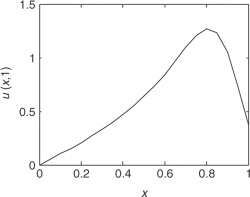
where α = 1.2, d(x) = 0.1x2.4 and q(x, t)=sin x is independent of time. shows the numerical solution to the governing equation with the conditions (28) at the time T = 1. For the inverse source problem, the corresponding additional condition is
(m = 1, … N), where N = 1/Δx, Δx = Δt = 0.05, i.e.
and the set of basis functions
is selected.
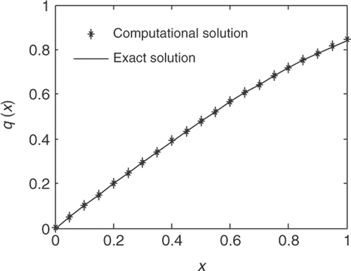
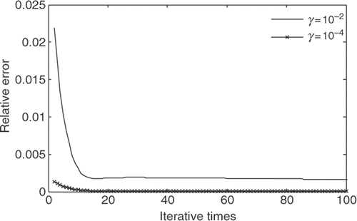
First, we choose the initial guess function as q0(x) = 1 + x + x2, and the regularization parameters as γ = 10−2 and γ = 10−4, respectively. shows the comparison of the computational solution to the exact solution of the source term. It is obvious that the computational solution matches well with the exact solution in this case. Through comparing the data in and , we know that the parameter vector is stable after iterating more than 4000 times with γ = 10−2, but the convergent rate is slower than the regularization parameter 10−4. Note that the relative error is less than 10−4 after iterating several times, and then it reaches the level of 3.7671 × 10⁻⁵. shows the relative errors of different regularization parameters at each iterative step.
Table 1. Comparing the data of q0(x) = 1 + x + x2 and γ = 10−2.
Table 2. Comparing the data of q0(x) = 1 + x + x2 and γ = 10−4.
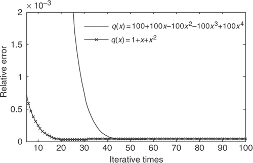
Choosing another initial guess function as q0(x) = 100 + 100x − 100x2 − 100x3 + 100x4 and the regularization parameter as γ = 10−4, and comparing the data in and , we can see that the convergent rate in this case is slower than the first one. shows the relative errors of different initial guess functions at each iterative step.
Table 3. Comparing the data of q0(x) = 100 + 100x−100x2−100x3 + 100x4 and γ = 10−4.
The results show that the relative error gets the level of 3.7671 × 10⁻⁵ and the parameter vector K is [0.0000, 0.9992, 0.0057, −0.1824, 0.0189]. shows the computational solution matches well with the exact solution.
Example 2
The governing equation
(29)
with the initial and boundary conditions
(30)
where the fractional derivative order α = 1.8, the diffusion coefficient d(x) = 1 and the source term
In order to estimate the source term, we select the set of basis functions
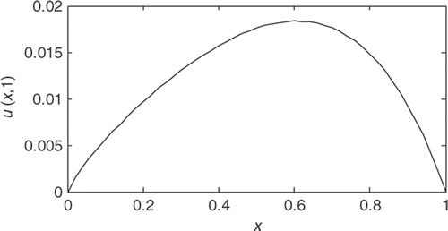
the regularization parameter γ = 10−7, the iterative step Δx = Δt1/N = 1/50 and the initial guess vector K0 = [1, 1, 1, 1, 1]. The additional condition is u (x, 1). shows the numerical solution to the governing equation with the initial and boundary conditions (30) at the time t = T.
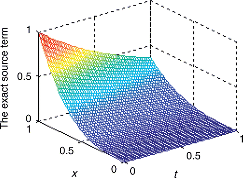
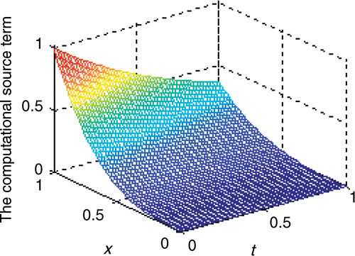
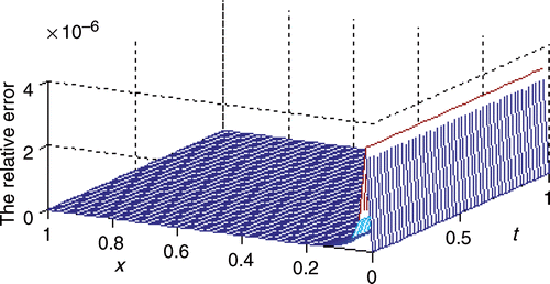
From , we can see that the computational solution K = [0.0000, −0.0000, 0.0000, 1.0000, 0.0000] matches well with the exact solution in this study. and show the exact solution and the computational solution to the source term, respectively. shows that the relative error is less than 4 × 10⁻⁶ after iterating 800 times at each point.
Table 4. Comparing the data of q0(x, t) = e−t + xe−t + x2e−t + x3e−t + x4e−t and γ = 10−7.
4. Conclusions
In this article, we present a coupled method based on the best perturbation method to solve the inverse source problem of one-dimensional spatial fractional diffusion equation on a finite domain. The coupled method is stable and easy to programme in this studied numerical examples, but the stabilization of the coupled method, the initial guess function and basis functions are closely related. A complete proof of the stabilization of the coupled method is our focus in future research work.
Therefore, some open issues still require further research:
| 1. | Basis functions play a key role in the coupled method. Due to the unknown properties of source terms, it is difficult to choose a set of basis functions. In general, we select basis functions by experience. This issue is short of theoretical analysis. | ||||
| 2. | Because the regularization parameter has a significant impact on the convergence rate, it is important to choose an appropriate regularization parameter. It needs further research, though there are some methods presented by predecessors Citation21–24. | ||||
| 3. | The initial guess function also has a significant impact on the convergent rate. The irrational selection of the function may lead to wrong results. For the coupled method, the initial guess function is chosen as an approximation of the exact solution. Actually, the exact solution cannot be known in advance and even all of its properties are unclear. We will do further research on this issue | ||||
Acknowledgements
This research is partially supported by the Program for New Century Excellent Talents in University, China (Grant no. NCET-06-0480).
References
- Chen, W, 2006. A speculative study of 2/3-order fractional Laplacian modeling of turbulence: Some thoughts and conjectures, Chaos 17 (2006), pp. 023126–023126.
- Wang, S, Ma, ZF, and Yao, HQ, 2008. Fourier-Bessel series algorithm in fractal diffusion model for porous material, Chin. J. Comput. Phys. 25 (2008), pp. 289–295.
- Tong, SJ, Zheng, W, and Chen, BZ, 2006. Analysis of the pollution consequences on leakage and seepage flow of poisonous liquid, Ind. Saf. Environ. Prot. 32 (2006), pp. 56–58.
- Sun, HG, Chen, W, and Chen, Y, 2009. Variable-order fractional differential operators in anomalous diffusion modeling, Physica A, 388 (2009), pp. 4586–4592.
- De Andrade, MR, Lenzi, EK, Evangelista, LR, Mendas, RS, and Malacarne, LC, 2005. Anomalous diffusion and fractional diffusion equation: Anisotropic media and external forces, Phys. Lett. A, 347 (2005), pp. 170–179.
- Podlubny, I, 1999. Fractional Differential Equations. San Diego: Academic press; 1999.
- Prakash, AO, 2004. Application of fractional derivatives in thermal analysis of disk brakes, Nonlinear Dyn. 38 (2004), pp. 191–206.
- Depollier, C, Fellah, ZEA, and Fellah, M, 2004. Propagation of transient acoustic waves in layered porous media: Fractional equations for the scattering operators, Nonlinear Dyn. 38 (2004), pp. 181–190.
- Cresson, J, 2010. Inverse problem of fractional calculus of variations for partial differential equations, preprint. Commun. Nonlinear Sci. Numer. Simulat. 15 (2010), pp. 987–996.
- Battaglia, JL, Cois, O, Puigsegur, L, and Oustaloup, A, 2001. Solving an inverse heat conduction problem using a non-integer identified model, Int. J. Heat Mass Transf. 44 (2001), pp. 2671–2680.
- Murio, DA, 2007. Stable numerical solution of a fractional-diffusion inverse heat conduction problem, Comput. Math. Appl. 53 (2007), pp. 1492–1501.
- Murio, DA, 2008. Time fractional IHCP with Caputo fractional derivatives, Comput. Math. Appl. 56 (2008), pp. 2371–2381.
- Sivaprasad, R, Venkatesha, S, and Manohar, CS, 2009. Identification of dynamical systems with fractional derivative damping models using inverse sensitivity analysis, CMC, 298 (2009), pp. 1–29.
- Metzler, R, and Klafter, J, 2004. The restaurant at the end of the random walk: Recent developments in the description of anomalous transport by fractional dynamics, J. Phys. A: Math. Gen. 37 (2004), pp. 171–208.
- Meerschaert, MM, and Tadjeran, C, 2004. Finite difference approximations for fractional advection-dispersion flow equation, J. Comput. Appl. Math. 172 (2004), pp. 65–77.
- Meerschaert, MM, and Tadjeran, C, 2006. Finite difference approximations for two-sided space-fractional partial differential equations, Appl. Numer. Math. 56 (2006), pp. 80–90.
- Tadjeran, C, Meerschaert, MM, and Scheffler, H-P, 2006. A second-order accurate numerical approximation for the fractional diffusion equation, J. Comput. Phys. 213 (2006), pp. 205–213.
- Gol’dman, NL, 2005. Determination of the right-hand side in a quasilinear parabolic equation with a final observation, J. Differ. Eqns 41 (2005), pp. 384–392.
- Golub, GH, Hansen, PC, and Leary, DPO, 1999. Tiknonov regularization and total least square, Siam J. Matrix Anal. Appl. 21 (1999), pp. 185–194.
- Peng, Y-M, , Research on numerical methods of the inverse problem for partial differential equations, Ph.D. diss., Xi’an University of Technology, 2004.
- Morozov, VA, 1966. On regularization of ill-posed problems and selection of regularization parameter, J. Comput. Math. Math. Phys. 6 (1966), pp. 170–175.
- Tikhonov, AN, and Arsenin, VY, 1977. Solution of Ill-posed Problems. New York: John Wiley & Sons; 1977.
- Engl, HW, 1987. Discrepancy principles for Tikhonov regularization of ill-posed problems leading to optimal convergence rates, J. Optim. Theory Appl. 52 (1987), pp. 209–215.
- Groesch, CW, 1984. The Theory of Tikhonov Regularization for Fredholm Equations of the First Kind. London: Pitman Advanced Publishing Program; 1984.
