Abstract
This study is motivated by a desire to obtain a numerical approach combining the use of the finite difference method with the solution of ordinary differential equation proposed for the determination of unknown coefficient in an inverse heat conduction problem. To regularize the resultant ill-conditioned linear system of equations, we apply the Tikhonov regularization method to obtain the stable numerical approximation to the solution.
1. Introduction
The problem of determining unknown coefficients in parabolic partial differential equations has bean treated by many authors. Usually these problems involve the determination of a single unknown parameter from overspecified boundary data. In some applications, however, it is desirable to be able to determine more than one parameter from the given boundary data Citation1–9.
When the radiation of heat from a solid is considered to pass through a nonparticipating media, the heat flux is often taken to be proportional to the difference of the boundary temperature of the solid to the fourth power and the temperature of the surroundings to the fourth power Citation1. When the thermo-physical properties are independent of position and temperature, the heat transfer problem in this situation may be derived, in the dimensional space and time, as
(1)
(2)
(3)
(4)
where T is a given constant, r(x) is the initial temperature of solid and φ(U(0, t)) + ζ(t) and ψ(U(1, t)) + η(t) represent a general radiation law. In this context the functions ζ(t) and η(t) are known heat fluxes arriving to the surfaces at x = 0 and x = 1, respectively, and the nonlinear terms φ(U(0, t)) and ψ(U(1, t)) are unknown functions to be determined with respect to the following overspecified conditions:
(5)
If the functions φ and ψ are given, then there may be no solution for an over specified problem (1–5). On the other hand, when φ and ψ are known, a priori, there exists a unique solution for the problem (1–4) and this solution may not satisfy the overspecified conditions (5), as in Citation14. In the problem (1–5), if the functions φ and ψ are unknown, one deals with an inverse heat transfer problem. In this case, we say that the pair of functions (U, (φ, ψ)) provides a solution to the inverse problem (1–5). The theoretical discussion is well-addressed in Citation4. This study focuses on the numerical method.
2. Overview of the numerical method
To solve the inverse problem (1–5), let us consider the following auxiliary inverse problem:
(6)
(7)
(8)
(9)
and the overspecified conditions
(10)
where U0(x) = r(x) and p(t) and q(t) are unknown functions. To provide a solution to the inverse problem (6–10), the additional information (10) should be considered. The temperature histories at some locations are measured in a slab. It is assumed that M thermocouples are used to record the temperature information at selected locations. Temperature histories taken from the thermocouples at successive specific dimensionless time tk are denoted by Ui,k for i = 1, 2, … , M and k = 1, 2, … , N, where N denotes the number of the discrete measurement times.
The application of the present numerical method to find the solution of problem (6–10) can be described as follows:
To remove time dependent terms in problem (6–9), one may replace the time derivative of temperature in Equation (6) with the first backward finite difference formula. After some evaluation, the following problem can be derived:
(11)
(12)
(13)
where Uk(x) = U(x, kΔt), 0 < x < 1 with
being a dimensionless time step,
The problem (11–13) is a two-point boundary-value problem and the prescribed conditions (12) and (13) are called the boundary conditions.
Theorem 1
Let Uk−1(x), be continuous on [0, 1]. Then the boundary-value problem (11–13) has a unique solution for any constants pk and qk, Citation10.
The analytical unique solution of problem (11–13) is as follows:
(14)
where
(15)
(16)
and
(17)
Now, writing Equation (14) for M points yields the following algebraic system of equations with two unknowns, pk and qk
(18)
where
, i = 1, … , M, represent the measured temperature taken from the M thermocouples at the location xi for i = 1, … , M, at the successive specific dimensionless time tk and
(19)
Remark 1
When M = 2, the system of equations (18) has a unique solution.
Proof
We must prove that the
Now, if the determinant of A is equal to zero then
and finally
therefore x1 = x2. This is impossible, since x1 ≠ x2. Thus the assumption that the det(A) = 0 leads to a contradiction.
Remark 2
When M > 2, it becomes an overdetermined system that can be solved in a sense of minimization of a criterion function (linear least-squares method). Let
describe this function.
To obtain the minimum value of Sk with respect to pk and qk, differentiation of Sk with respect to pk and qk will be performed.
In matrix form, the values of pk and qk can be obtained from solving the following matrix equation:
(20)
where
and
Therefore the following system is obtained
(21)
and (ATA)−1AT is the reverse matrix of the inverse problem.
Remark 3
The matrix ATA is invertible.
Using the Cauchy–Schwartz inequality and Remark 1 yields
2.1. Regularization method
Mathematically, IHCPs belong to the class of ill-posed problems. As a consequence, large-amplitude changes at the surface have to be inferred from small-amplitude changes in the measurements data. Errors and noise in the data can therefore be mistaken as significant variations of the surface state by the estimation procedure. Since the matrix A is ill-conditioned, the solution of Equation (20) can be corrupted by an amplified propagation of the data noise, so that regularization methods must be used for controlling this noise propagation. In our computation, we adapt the Tikhonov regularization method Citation11 to solve the matrix equation (18).
Definition
Let A ∈ Rm×n be a matrix and let m ≥ n, then the singular value decomposition (SVD) of A is defined by
where
and
, are orthogonal matrix with orthogonal columns, ui and vi are the left and right singular vectors of A, respectively and S ∈ Rn×n is a diagonal matrix where diagonal elements appearing in nonincreasing order of nonnegative singular values σ1 ≥ σ2 ≥ ··· ≥ σn ≥ 0. In case m < n, then define the SVD from AT.
Now for ,
and
Note
The Tikhonov regularized solution to the system of linear algebraic equation is given by (Θk)α, where
(22)
The quasi-optimality criterion is used to determine a suitable value of α Citation12,Citation13.
For evaluating φ and ψ we use
(23)
(24)
Therefore
(25)
(26)
Finally, the MATLAB package is used for interpolating these values and reconstructing the functions φ and ψ.
3. Numerical results and discussion
In this section, we are going to illustrate numerically, some of the results for two unknown boundary conditions in the inverse problem (1–5). All the computations are performed on the PC (pentium(R) 4 CPU 3.20 GHz).
Example 1
In this example let us consider the following inverse problem:
(27)
(28)
(29)
(30)
with the overspecified conditions
(31)
The exact solution of this problem is U(x, t) = x2 + 2t, φ(U(0, t)) = sin((U(0, t))2 + 1) and ψ(U(1, t)) = cos((U(1, t))2 + U(1, t)).
and show the comparison between exact and approximate solutions results from the regularization method and the pseudoinversion method with noiseless data for the problem (27–31). In addition for this problem, and show the comparison between exact and foregoing approximate solutions with discrete noisy data (noisy data = input data + (0.01)rand(1)).
Table 1. The values of φexact, φregularization method and φpseudoinversion method in t = jΔt for the problem (27–31) with noiseless data when Δt = 0.01 and xi = 0.6, 0.7, 0.8.
Table 2. The values of ψexact, ψregularization method and ψpseudoinversion method in t = jΔt for the problem (27–31) with noiseless data when Δt = 0.01 and xi = 0.6, 0.7, 0.8.
Table 3. The comparison between φexact, φregularization method and φpseudoinversion method in t = jΔt for the problem (27–31) with noisy data when Δt = 0.025 and xi = 0.88, 0.90, 0.92.
Table 4. The comparison between ψexact, ψregularization method and ψpseudoinversion method in t = jΔt for the problem (27–31) with noisy data when Δt = 0.025 and xi = 0.88, 0.90, 0.92.
Example 2
In this example let us consider the following inverse problem:
(32)
(33)
(34)
(35)
with the overspecified conditions
(36)
The exact solution of this problem is U(x, t) = exp(−t)cos(x), φ(U(0, t)) = (U(0, t))2 and ψ(U(1, t)) = (U(1, t))2 + U(1, t).
Tables show the comparison between exact and approximate solutions for the problem (32–36) with noiseless data and discrete noisy data (noisy data = input data + (0.01)rand(1)), respectively.
Furthermore, Figures show the difference between the exact and approximate results using regularization method and pseudoinversion method with noiseless data and discrete noisy data for φ(U(0, kΔt)) and ψ(U(1, kΔt)).
Figure 1. Difference between the φexact, φregularization method and the φexact, φpseudoinversion method of the problem (27–31) with noiseless data.
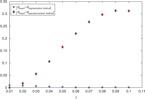
Figure 2. Difference between the ψexact, ψregularization method and the ψexact, ψpseudoinversion method of the problem (27–31) with noiseless data.
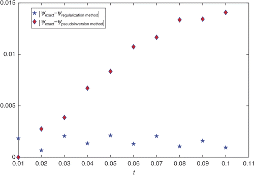
Figure 3. Difference between the φexact, φregularization method and the φexact, φpseudoinversion method of the problem (27–31) with noisy data.
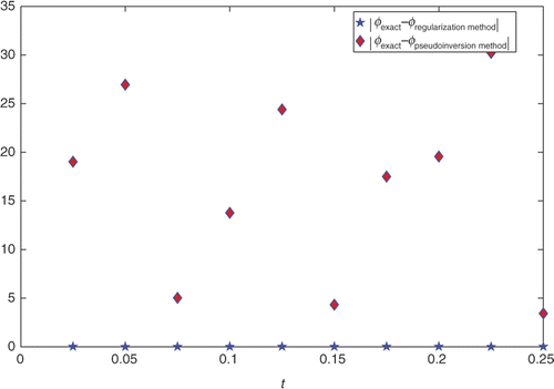
Figure 4. Difference between the ψexact, ψregularization method and the ψexact, ψpseudoinversion method of the problem (27–31) with noisy data.
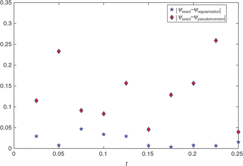
Figure 5. Difference between the φexact, φregularization method and the φexact, φpseudoinversion method of the problem (32–36) with noiseless data.
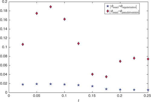
Figure 6. Difference between the ψexact, ψregularization method and the ψexact, ψpseudoinversion method of the problem (32–36) with noiseless data.
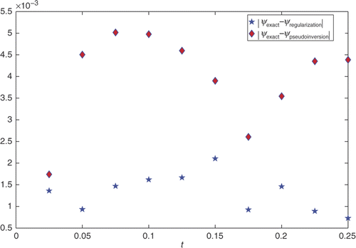
Figure 7. Difference between the φexact, φregularization method and the φexact, φpseudoinversion method of the problem (32–36) with noisy data.
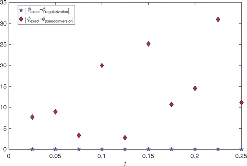
Figure 8. Difference between the ψexact, ψregularization method and the ψexact, ψpseudoinversion method of the problem (32–36) with noisy data.
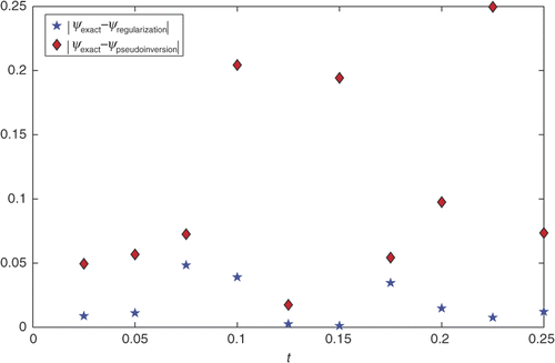
Table 5. The values of φexact, φregularization method and φpseudoinversion method in t = jΔt for the problem (32–36) with noiseless data when Δt = 0.025 and xi = 0.7, 0.8, 0.9.
Table 6. The values of ψexact, ψregularization method and ψpseudoinversion method in t = jΔt for the problem (32–36) with noiseless data when Δt = 0.025 and xi = 0.7, 0.8, 0.9.
Table 7. The comparison between φexact, φregularization method and φpseudoinversion method in t = jΔt for the problem (32–36) with noisy data when Δt = 0.025 and xi = 0.88, 0.90, 0.92.
Table 8. The comparison between ψexact, ψregularization method and ψpseudoinversion method in t = jΔt for the problem (32–36) with noisy data when Δt = 0.025 and xi = 0.88, 0.90, 0.92.
References
- Cannon, JR, 1984. The One-Dimensional Heat Equation. Reading, MA: Addison Wesley; 1984.
- Beck, JV, Blackwell, B, and Clair, Ch.R.St., 1985. Inverse Heat Conduction. New York: John Wiley and Sons; 1985.
- Cannon, JR, and Zachmann, D, 1982. Parameter determination in parabolic partial differential equations from overspecified boundary data, Int. J. Eng. Sci. 20 (1982), pp. 779–788.
- Shidfar, A, and Azary, H, 1997. Nonlinear Parabolic Problems, Nonlinear Analysis, Theory, Methods Appl. 30 (8) (1997), pp. 4823–4832.
- Cannon, JR, and Lin, Y, 1988. Determination of parameter p(t) in some quasi-linear parabolic differential equations, Inverse Probl. 4 (1988), pp. 35–45.
- Lin, Y, 1994. Analytical and numerical solution for a class of nonlocal nonlinear parabolic differential equations, SIAM. J. Math. Anal. 25 (1994), pp. 1577–1594.
- Shidfar, A, Pourgholi, R, and Ebrahimi, M, 2006. A numerical method for solving of a nonlinear inverse diffusion problem, Comput. Math. Appl. 52 (2006), pp. 1021–1030.
- Ebrahimian, M, Pourgholi, R, Emamjome, M, and Reihani, P, 2007. A numerical solution of an inverse parabolic problem with unknown boundary conditions, Appl. Math. Comput. 189 (1) (2007), pp. 228–234.
- Pourgholi, R, Azizi, N, Gasimov, YS, Aliev, F, and Khalafi, HK, 2009. Removal of numerical instability in the solution of an inverse heat conduction problem, Commun. Nonlinear Sci. Numer. Simul. 14 (6) (2009), pp. 2664–2669.
- Myint-U, T, 1978. Ordinary Differential Equations. New York: Elsevier North-Holland; 1978.
- Tikhonov, AN, and Arsenin, VY, 1977. On the Solution of Ill-posed Problems. New York: Wiley; 1977.
- Fierro, RD, and Bunch, JR, 1994. Collinearity and total least squares, SIAM J. Matrix Anal. Appl. 15 (1994), pp. 1167–1181.
- Morozov, VA, 1984. Methods for Solving Incorrectly Posed Problems. New York: Springer-Verlag; 1984.
- Friedman, A, 1964. Partial Differential Equations of Parabolic Type. Englewood-Cliffs, NJ: Prentice-Hall; 1964.