Abstract
Model calibration is an inverse problem in which unknown model parameters are to be inferred from test data. Due to the ill-posed characteristics of inverse problems, model calibration is a challenging problem. This article presents an inverse method based on the statistical inverse theory. In this method multiple formulations for calibration are used simultaneously, and their results are averaged according to how likely each formulation is. The inverse method is applied to calibration of a computer model of a turbojet engine. It is demonstrated that the method accurately estimates the model parameters with limited amount of noisy data. It is also demonstrated that the method is capable of identifying possible alternative solutions and that using multiple competing formulations gives rise to more accurate and conclusive results than using single general formulation.
1. Introduction
In many engineering disciplines it is often desirable to calibrate computer models to test data. Unlike analyses in which physical properties are predicted with given model parameters, model calibration is an inverse problem in which unknown model parameters are to be estimated from test data. Numerous techniques have been developed to solve inverse problems. However, solving inverse problems is still challenging due to their ill-posed characteristics. Inverse problems often do not have a unique solution, and their solutions are sensitive to errors in data, modelling and computation Citation1. The following sections survey various estimation techniques and present a novel inverse method based on the statistical inversion theory. The inverse method is applied to calibration of a computer model of a turbojet engine, and its accuracy is evaluated.
2. Model calibration
Consider a model that maps a vector of model parameters x to a vector of measurable variables y. This mapping can be written as
(1)
where f is a nonlinear function, and ϵ is a vector of sensor random noise. The random noise of each measurable variable is generally assumed to follow a Gaussian distribution with zero mean and a constant variance. The difference between y and f(x) is called residual. To calibrate the model to y, the vector of model parameters x must be adjusted such that the residual is negligible. The nonlinear least squares method finds x that minimizes the sum of squared residuals. Unfortunately, the nonlinear least squares method does not have a closed form solution and is usually solved with an iterative approach. Most iterative approaches require initial values, and their convergence is not guaranteed.
If the nonlinear function f can be linearized without any significant loss of accuracy, one can use one of the linear techniques from the various ones that have been researched in so many years. The linearized model can be written in matrix form such as
(2)
Here, unlike in Equation (1), ϵ includes not only the sensor random noise but also linearization error. The simplest, but not necessarily the most effective, way to solve Equation (2) is to invert the matrix A:
(3)
However, Equation (3) is valid only if A is invertible, i.e. A is a nonsingular square matrix. In many cases the matrix A is rank-deficient because measurements are often fewer than model parameters.
When A is not invertible, the method of least squares is commonly used to solve the system of linear equations Citation2. The method of least squares finds x that minimizes the sum of squared residuals
(4)
In the method of least squares each measurement has the same importance to the objective function JLS no matter how accurate each sensor is. In reality, however, each sensor has different precision, and it may be reasonable to weigh precise measurements more than imprecise ones. The method of weighted least squares finds x that minimizes
(5)
where R is the covariance matrix of the error ϵ. These two methods are sensitive to errors in the measurement vector y because the residual (y − Ax) is squared in their objective functions.
Singular value decomposition (SVD) is an alternative to the least squares method for solving the system of linear equations y = Ax. The SVD decomposes the matrix A and determines the pseudo-inverse A† of A. The SVD solution of the system of linear equations is A†y. It is the minimum norm, least squares solution of the system of linear equations Citation3. In practice, to reduce adverse effects of singular values close to zero, such singular values are often replaced with zero. The SVD with this modification is called the truncated SVD Citation3.
The methods surveyed thus far result in a point estimate. These methods provide neither the confidence in the point estimate nor any information on the solution space that might contain multiple solutions. A rigorous statistical approach dealing with probability distributions is needed to reveal the full information of the solution space. The statistical inversion theory recasts an estimation problem to a statistical inference problem. In this approach all variables are treated as random variables, each following a probability distribution. The forward mapping from the unknowns x to the measurable variables y can be probabilistically modelled from the relation between x and y. This mapping is represented by a conditional probability p(y|x). In addition, the analyst or domain expert can have a prior knowledge on the vector of model parameters x, and the prior knowledge can be transformed to a prior probability p(x). When some measurements y are made, the probability of x can be updated. The updated probability p(x|y) is called the posterior probability, which is of primary interest of the statistical inversion theory. Bayes' rule links the conditional probability and the posterior probability, written as
(6)
Once the posterior distribution is known, point estimates can be obtained from the posterior. Most popular point estimates are a conditional mean (CM) and a maximum a posterior (MAP) estimate Citation3:
(7)
(8)
3. A Bayesian model averaging inverse method
This article presents a Bayesian method, based on the statistical inversion theory, that solves Y = AX + ϵ to find X, given Y and A. X and Y are independent and dependent variables, respectively, and A is a matrix of coefficients. Unlike Equation (2), the variables are capitalized because each of them is treated as a random variable following a probability distribution. Instances of the random variables will be in lower case.
3.1. Conditional probability p(Y|X)
Let us assume that ϵ is random noise following a Gaussian distribution with zero mean and a constant precision matrix τ, which is an inverse of a covariance matrix. Subsequently, given X, the probability of Y follows a Gaussian distribution with a mean vector and the precision matrix τ. The mean vector μ can be written as
(9)
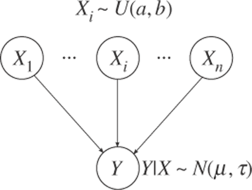
where Xi is the i-th element of X, ai is a column vector of A, and n is the size of X. Xi can be any value within a range of interest. If no particular value of Xi is preferred over others, a uniform distribution can be used for the prior distribution of Xi. This model can be shown graphically as in . Each node represents a random variable, and each edge represents probabilistic dependency between two nodes. ai is the strength of the edge between Xi and Y except for a0, which is the interceptor.
With limited data or knowledge the precision matrix τ is often unknown. Thus, τ is considered as a variable that is to be inferred from data. The vague knowledge on τ can be modelled with a non-informative, disperse prior. A conjugate prior of the precision matrix of a multivariate normal distribution is an Wishart distribution W(Λ, ν) where Λ is the scale matrix, and ν is the degree of freedom Citation4. The elements of Λ are set so as to make the Wishart distribution disperse.
While building a graphical model like the one shown in , it is important to take sparsity into consideration. Depending on instances of Y, it may not be necessary to include all elements of X. Even though the model with the full vector X is the most general so that it can be applied to any instances of Y, its accuracy is not as good as that of the model tailored to the particular instances of Y. The tailored model includes only the necessary elements of X. This is the same issue as variable selection in linear regression. In both cases one needs to search for the best model to fit the data on hand. To make the search process efficient, the spike and slab distribution Citation5 is used for X as described next.
3.2. Probability of X
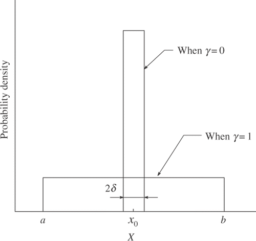
The spike and slab distribution is a combination of two uniform distributions, the taller and narrower spike, and the shorter and wider slab, as shown in . Choice between the two depends on an auxiliary binary variable vector γ. Each element of γ is connected to each element of vector X. When γi is equal to zero, the associated Xi follows the spike so that it is likely to be fixed at a pre-defined value x0. When γi is equal to one, Xi can be any value in the range of [a, b]. The resulting probability distribution for Xi is written as
(10)
where δ is a small constant.
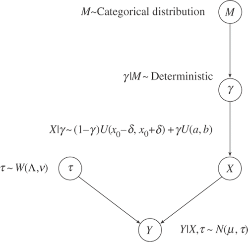
As the elements in γ change from zero to one or vice versa, the associated elements of X are included or excluded from the system of linear equations and, subsequently, from the graphical model. The total number of possible models is 2n. A categorical variable M is introduced to represent these 2n models. Unless there is a sufficient reason to favour one model over another, it is reasonable to use a non-informative prior Citation6; each model is equally probable. Thus, a categorical distribution with 2n categories is assigned to the model variable M such that the probability of M being a particular model m is as follows:
(11)
The assumption of equally probable models is equivalent to assigning
(12)
for all i. M and γ are added to the graphical model in , and the resulting graphical model is shown in . The elements in A are constant and does not change with the model. Therefore, it is not shown in the graphical model.
3.3. Posterior probability p(X|Y)
The ultimate goal of using the graphical model in for the calibration problem is to determine posterior distribution of variables of interest such as X and M when some instances of Y become available. The posterior probability of X, p(X|Y), can be expanded using marginalization as follows:
(13)
p(X|Y, m) is the posterior of X when the model variable M is equal to m. p(m|Y) is a number between zero and one, and the summation of p(m|Y) over all models is equal to one. Therefore, Equation (13) is merely the average of the posterior of X from each model using the model posterior p(m|Y) as a weighting factor. This is why the current method is called Bayesian model averaging (BMA; Citation7). Equation (13) can be further derived using Bayes' rule as follows:
(14)
where p(m) is the prior probability of the model variable M being a particular model m. Because X, Y and M constitute a serial connection, and X is in the middle of the serial connection, Y is independent of M given X Citation8. Therefore, the first factor in Equation (14) can be written as
(15)
The second factor p(X|m) can be written using marginalization as follows:
(16)
p(γ|m) is one if the model m includes X and zero otherwise. Now the posterior distribution p(X|Y) is expressed with all known CPDs defined in Sections 3.1 and 3.2.
A degree to which each model is supported by data is determined by the model posterior p(M|Y), which can be expressed with the CPDs using Bayes' rule and marginalization as follows:
(17)
p(Y|x) and p(x|M) are given in Equations (15) and (16), respectively. Even though Equations (14) and (17) are derived up to proportionality instead of equality, the posterior distributions still can be uniquely determined using the fact that any proper probability distribution integrates to one.
3.4. Calculation of the posteriors
Calculation of the posterior distributions involves the multidimensional integrations of the possibly multimodal functions. Because the integrands are not derivable analytically, the posteriors are calculated approximately using the Gibbs sampler. A general description of the Gibbs sampler is briefly described next. Consider a pair of random variables A and B. The Gibbs sampler generates a sample from a marginal probability distribution p(A) by sampling from conditional probability distributions p(A|B) and p(B|A) alternately as follows Citation9:
(18)
Starting from an arbitrary initial value b0, if the sampling repeats for a large number k, ak is effectively a sample from p(A). For this study a Gibbs sampling software in public domain WinBUGS Citation10 is used for calculating the posterior distributions.
The use of a sampling technique is crucial to the scalability of the current method. The number of possible models doubles as the number of model parameters, n, increases by one. Subsequently, the categorical model variable M can easily have a large number of categories. A combinatorial approach cannot be applied to this problem if n is too large and, subsequently, there are too many models, or subsets of model parameters. Unlike combinatorial approaches, the Gibbs sampling does not visit all the models. In this Bayesian formulation it is automatically determined which models will be visited more often than others. The large number of models adds significantly less computational burden to the Gibbs sampler than to a combinatorial approach.
4. Test case
As a proof-of-concept the BMA inverse method is applied to calibration of a computer model of a turbojet engine to simulated test data. The computer model is the numerical propulsion system simulation (NPSS) Citation11 developed by NASA. In this test case seven parameters in NPSS are calibrated using five measurements. The NPSS parameters and measurements are listed in . The nonlinear computer model NPSS is approximated by a system of linear equations Y = AX. To determine the matrix A, a design of experiment (DOE) is built using NPSS simulations with all model parameters in the range of [0.96, 1.02] except for the nozzle gross thrust coefficient, which is in the range of [0.95, 0.99]. The engine operating condition is fixed at the sea level. For each measurable variable a first order polynomial equation is created as a function of the seven NPSS parameters. The coefficients of the linear polynomial equations constitute the matrix A, and the resulting equations are written in matrix form as
(19)
Table 1. NPSS parameters and measurable variables.
To generate simulated test data, NPSS is run with a pre-defined set of the parameters. The compressor efficiency and flow scalars are set to 0.98, and every other parameters to 1, which is the default value. To simulate random noise in actual engine test data, random numbers generated from Gaussian distributions are added to the NPSS output of the six measurable variables. The variances of the Gaussian distributions are set to 1% of the NPSS output at the sea level operating condition.
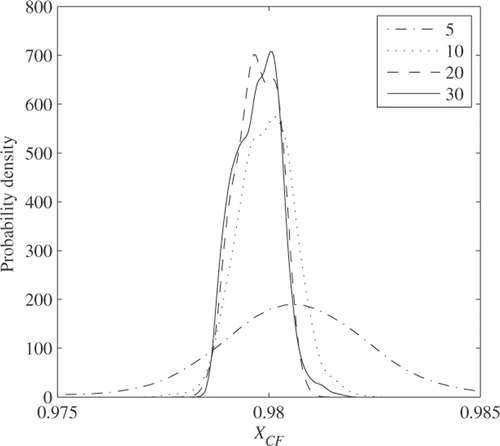
The BMA inverse method is capable of analysing multiple data points obtained at different instants of time all together. A solution from the BMA inverse method varies with the number of data points. To find a proper number of data points for the test case, the BMA inverse method is applied to the case with various numbers of data points. shows the posterior of XCF with various numbers of data points. As the number of data points increases, the posterior probability distribution becomes concentrated around the true value 0.98. Since the probability distribution changes little with more than the 20 data points, it can be said that the solution converges with the 20 data points in this test case. The results presented hereafter are from the 20 data points. Please note that the convergence is determined based on not only XCF but also on all other variables not shown here. If the number of data points is not large enough for convergence to be achieved, the intermediate posterior probability distributions can lead to the right solution with low confidence. However, they can also lead to inaccurate or wrong point estimates.
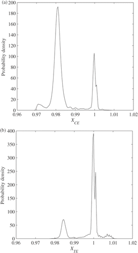
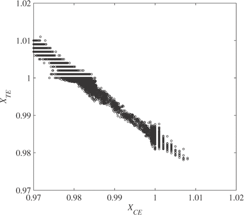
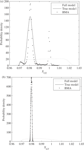
With the 20 data points all the scalars except for XCE and XTE have a unimodal posterior concentrated near their true value. The multimodal posteriors of XCE and XTE are shown in . The posterior of XCE has two modes near the true value 0.98 and one. The posterior of XTE has two modes near the true value one and 0.985. They are multimodal because multiple models in various forms are considered. Some models contribute to one mode while others do to the other. The multimodal posteriors of XCE and XTE suggest that multiple pairs of {XCE, XTE} can possibly result in the 20 data points: {1, 1}, {1, 0.985}, {0.98, 1}, and {0.98, 0.985}. It is necessary to determine which pair is more likely as compared with the others. shows the bivariate scatter plot of the Gibbs samples in the two dimensional space constituted by the two scalars. The two scalars appear to be strongly correlated, and there is no Gibbs sample near {1, 1} and {0.98, 0.985}. It can be said that these two pairs are unlikely to happen. By contrast, the cloud of the Gibbs sample passes the other two pairs, {1, 0.985} and {0.98, 1}. In fact, extra NPSS runs with the two pairs {1, 0.985} and {0.98, 1} revealed that they result in nearly the same NPSS outcome when all other scalars are the same. This insignificant difference cannot be distinguished due to the sensor noise and the linearization error. With the five measurable variables listed in , it is difficult to decide which of XCE and XTE should be selected to calibrate NPSS to the test data.
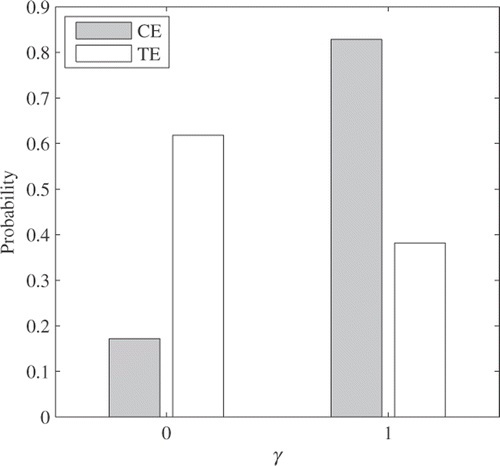
Between the two remaining pairs, a decision on which pair is more likely can be made by investigating the posterior of γ. Since the number of the model parameters is seven, total 27, or 128, models are considered in this test case. Initially the two states of γ, zero and one, are equally likely to be true. Once some data are given some models are much more supported by the data than others. γ becomes more likely to be one if the corresponding model parameter commonly appears in the supported models. shows the posteriors of γ associated with XCE and XTE. While γTE is more likely to be zero than one, γCE is 2.5 times more likely to be one than zero. It can be said that the compressor efficiency scalar is needed much more than the turbine efficiency scalar.
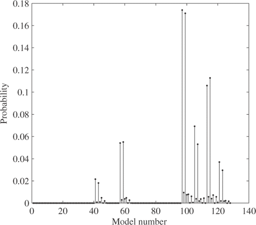
The posterior distributions of X and γ contain information of individual model parameters averaged over all the 128 models. The posterior of the model variable M depicts how well each model explains the data. shows the model posterior calculated with the 20 data points. Nearly half of the models results in zero probability so that they are not worth further consideration; they are hardly supported by the data. Among the other half only 12 models count as much as 90% of the model posterior probability. lists the posteriors of the 12 models and the model parameters that each model contains. The BMA inverse method ranks the model with the compressor efficiency and flow scalars as the one with the highest posterior. In fact, among the 128 models considered, this model form is closest to how the simulated measurements are generated using NPSS; the compressor efficiency and flow scalars are deviated from their default values. Hereafter, this model is referred to as the true model. The true model is followed by the one with the duct pressure drop scalar in addition to the two compressor scalars. The posterior probabilities of the first two models is different only by 0.4%. It means that the duct pressure drop scalar plays an insignificant role in these two models. The insignificance of the duct pressure drop scalar prevails in the rest of the models. The model with the third highest posterior includes the two compressor scalars and the burner pressure drop scalar, and it is followed by the one that additionally includes the duct pressure drop scalar. These four models described above commonly include the compressor efficiency and flow scalars. By contrast, the next eight models commonly include the compressor flow scalar and the turbine efficiency scalar instead of the compressor efficiency scalar.
Table 2. Top twelve models.
The two distinct groups of the models, the first four and the next eight in , confirm the possibility of the two different solutions identified earlier from the posteriors of X and γ. Because the models including the compressor efficiency and flow scalars are more highly ranked than the models including the compressor flow and turbine efficiency scalars, it can be concluded that the compressor efficiency and flow scalars are better explaining the data than the compressor flow and turbine efficiency scalars. This conclusion is consistent with the conclusion made previously based on the posterior of γ. The BMA inverse method provides the means of identifying all the probable solutions and ranks the solutions based on their probabilities.
Among the 128 models, the true model, which contains only the necessary model parameters, is definitely the most accurate because it has the function form closest to how the data is generated. By contrast, the full model, which contains the entire model parameters, is not usually as accurate as the true model but is the most general. To compare the BMA inverse method with the full and true models, shows the posteriors of the compressor efficiency and flow scalars from the three cases with the 20 data points. The true model results in the posteriors each of which peaks near the true value. By contrast, the full model results in the disperse posteriors for both scalars, which are not much different from their uniform prior distribution, due to the limited amount of the data. Last, but not least, the BMA inverse method approximates the true model fairly well with the 20 data points. The multimodal posterior of the compressor efficiency scalar should be further investigated as discussed earlier.
5. Conclusion
This article presents an inverse method for model calibration based on the statistical inversion theory and BMA. The method uses multiple calibration formulations tailored in order to result in solutions with varying sparsity. These solutions are averaged according to how likely each formulation is. The Gibbs sampling is used to calculate approximate posteriors. The BMA inverse method is applied to calibration of a turbojet engine model to simulated test data. In spite of fewer measurements than model parameters, the BMA inverse method accurately estimates the probability distributions of the model parameters with limited amount of noisy data. It is demonstrated that averaging multiple competing formulations gives rise to more conclusive results than using single general formulation when the amount of available data is limited. Unlike classical estimators that solve an optimization problem and result in a point solution, the BMA inverse method can identify multiple solutions if they exist as it deals with probability distributions instead of point estimates and multiple formulations are kept under consideration. In addition, the BMA inverse method provides the means to rank the multiple solutions in the order of how likely each of them is.
Acknowledgement
The authors thank Russell Denney, Damon Rousis and Jacob Chang of Georgia Institute of Technology for providing the NPSS turbojet model.
References
- Hadamard, J, 1952. Lectures on Cauchy's Problem in Linear Partial Differential Equations. New York: Dover; 1952.
- Sorenson, HW, 1970. Least-squares estimation: From Gauss to Kalman, IEEE Spectrum 7 (1970), pp. 63–68.
- Kaipio, J, and Somersalo, E, 2004. Statistical and Computational Inverse Problems. New York: Springer; 2004.
- Congdon, P, 2001. Bayesian Statistical Modelling. Chichester: Wiley; 2001.
- Mitchell, TJ, and Beauchamp, JJ, 1988. Bayesian variable selection in linear regression, J. Am. Stat. Assoc. 83 (1988), pp. 1023–1032.
- Jaynes, ET, 2003. Probability Theory: The Logic of Science. Cambridge: Cambridge University Press; 2003.
- Wasserman, L, 2000. Bayesian model selection and model averaging, J. Math. Psychol. 44 (2000), pp. 92–107.
- Charniak, E, 1991. Bayesian networks without tears, AI Mag. 12 (1991), pp. 50–63.
- Casella, G, and George, EI, 1992. Explaining the Gibbs sampler, Am. Stat. 46 (1992), pp. 167–174.
- Lunn, DJ, Thomas, A, Best, N, and Spiegelhalter, D, 2000. WinBUGS-A Bayesian modelling framework: Concepts, structure, and extensibility, Stat. Comput. 19 (2000), pp. 325–337.
- A.L. Evans, G.J. Follen, C.G. Naiman, and I. Lopez, Numerical propulsion system simulation's national cycle program, Tech. Rep. AIAA-1998-3113, American Institute of Aereonautics and Astronautics, Reston, VA (1998).
