A meshless method for reconstructing the heat source and partial initial temperature in heat conduction

Abstract

In this article, we use the method of fundamental solutions to reconstruct the heat source and part of the initial temperature simultaneously in one-dimensional heat conduction problem. This problem is ill-posed, thus a Tikhonov regularization method with generalized cross-validation criterion is applied to obtain a stable numerical solution. Numerical experiments for several examples show that the proposed method is reasonable and feasible.

Keywords:

• ill-posed problem
• the method of fundamental solution
• Tikhonov regularization method
• inverse source problem
• backward heat conduction equation

AMS Subject Classifications::

• 65N20
• 65N80

1. Introduction

In this article, a computational method for solving the inverse heat source and identifying the partial initial temperature is investigated. By using the fundamental solutions as basis functions, we give a global approximation scheme in both spatial and time domains. The stability and error analysis of the algorithm are presented together with numerical results.

The inverse heat source problem is ill-posed in the sense of Hadamard 1. So it has received considerable attention from many researchers in a variety of fields by using different methods. Backward heat conduction problems (BHCP) are also inverse problems which are investigated by many authors, such as the boundary element method (BEM) 2, the iterative BEM 3–6, the operator-splitting method 7, the implicit inversion method 8, the lattice-free high-order finite difference method (FDM) 9, the contraction group technique 10, the method of fundamental solutions (MFS) 11 and the backward group preserving scheme 12. A detail survey of the BHCP was provided by Chiwiacowsky and de Campos Velho 13. To the best of the author's knowledge, simultaneous reconstruction for the heat source and the initial temperature seems not to have been studied elsewhere.

In 14,15, Yi and Murio considered the problems of source term identification in one- and two-dimensional inverse heat conduction problems (IHCPs) by using the mollification method and a marching scheme. They obtained the temperature, heat flux and general source terms and gave the error analysis.

In 16, Yamamoto and Zou investigated the simultaneous reconstruction for the initial temperature and heat radiative coefficient. In that paper, the conditional stability of the inverse problem was first established.

Recently, Li et al. 17 obtained a conditional stability estimate by the Carleman estimate for the reconstruction of the initial temperature. They assumed that some measurement data of the temperature can be observed both in a subregion inside and on the boundary of the physical domain, and divided into two ill-posed problems to investigate.

The traditional mesh-dependent FDM and the finite element method (FEM) require dense meshes, and hence tedious computational time, to give a reasonable approximation to the solution of backward heat conduction or inverse source problems and suffers from numerically instable problems. The advantage of the BEM is reducing the computational time and storage requirement but the problem of numerical stability still persists.

In recent years, meshless methods, including the radial basis functions (RBF) method 18,19, the MFS 20,21 and the boundary knot method (BKM) 22,23, have attracted great attention in the scientific and engineering fields. Meshless methods emerge as a competitive alternative to mesh-dependent methods. These meshless methods require neither domain discretization as in the FEM and FDM, nor boundary discretization as in the BEM, thus they improve the computational effect and can be easily generalized to solve high-dimensional differential equations. The MFS has been extensively applied to deal with some engineering problems.

Kupradze and Aleksidze 24 is a very early work concerning the MFS paper, and the MFS has been developed by many mathematicians and scientists over the past 40 years. In the beginning, the MFS was mainly applied to solve direct problems, such as the solutions for potential problems by Mathon and Johnston 25, the exterior Dirichlet problem in acoustics by Kress and Mohsen 26, and the biharmonic problems by Karageorghis and Fairweather 27. In 1995, Chen 28 applied the MFS to solve the non-linear problems.

The most important advantage of the MFS is that it is an inherently meshless and integration-free scheme for solving various types of partial differential equations. In 29, the MFS was applied to solve the IHCP by Hon and Wei. Motivated by their works, some researchers applied this scheme to solve many inverse heat problems, such as BHCP in 11, the inverse source problems 30–33 and so on.

More recently, Yan et al. 32,33 used the MFS to solve the inverse time- and spacewise-dependent heat source problems. In their works, they used the Tikhonov regularization technique with the generalized cross-validation (GCV) criterion for choosing the regularization parameters. However, they gave the initial temperature as measurement data to obtain the heat source terms. In a real application, we may not know either the heat source or initial temperature, and so we have to reconstruct both of them. In our inverse problem, the data are taken at final value, while an unknown source is time-dependent and, in general, this formulation causes the difficulty for proving e.g. the uniqueness. Thus we discuss a special form source and see Equation (1). In paper 34, the authors calculated the partial initial temperature by using the MFS. Hence, the method is the same as ours, and the problem is analogous to ours. In this article, we try to obtain simultaneous reconstruction of the partial initial temperature and the heat source. In order to avoid the singularities about the time variable t, we introduce a time parameter T.

This article is organized as follows. In Section 2, we give the mathematical formulation of our proposed problem. The MFS is considered in Section 3. In Section 4, we introduce the Tikhonov regularization with GCV criterion to choose regularization parameters. In order to verify the efficiency and accuracy of our proposed method, we state some typical numerical examples in Section 5. Finally, Section 6 gives a conclusion.

2. Problem formulation

Consider the following heat conduction problem in which the heat source f(t) depends on time only: (1) under the Dirichlet boundary conditions (2) the final condition (3) and the partial initial condition (4) where u_l(t), g(x) and h₁(x) are given functions which satisfy the following compatibility conditions: and the functions u(x, t), f(t), h₂(x) are unknown.

Because BHCP and inverse heat source problem are both ill-posed (see Refs. 35,36 for details), the problem mentioned above is also ill-posed. Hence, in this article, we will use the MFS combined with Tikhonov regularization to solve our proposed problem. The methodology will be proposed in Sections 3 and 4.

3. The MFS

In this section, we apply the MFS to construct an approximate solution to the problem (1–4).

First of all, we use a transformation for f(t) as follows: (5) By using the transformation above, the non-homogeneous equation (1) can be transformed into the following homogeneous one: (6) where v(x, t) = u(x, t) − r(t).

Thus, (2–4) can be rewritten below as (7) (8) (9) (10) Using v(0, t_max) = −r(t_max) and substituting (7) into (8–10), we obtain the following parabolic problem: (11) (12) (13) (14)

The fundamental solution of Equation (11) is given by (15) where H(t) is the Heaviside function. Meanwhile, we suppose that T > t_max is a constant. Then, the following time shift function 29,37 (16) is a non-singular solution of Equation (11) in the domain (0, l) × [0, t_max].

Then, the fundamental solutions centred at the nodal points , i = 1, … , n + m + s, are given by (17) here, the source points can be chosen as Γ = Γ₁ ∪ Γ₂ ∪ Γ₃ by (18) (19) (20) where d₁, τ, d₂ > 0 are the fixed constants.

Followed by the idea of MFS for solving IHCP in 29,37 and BHCP in 11, an approximation solution v* to the problem (11) under the conditions (12–14) can be expressed by the following linear combination of basis functions: (21) where φ_i(x, t) are given by (17) and λ_i are unknown coefficients to be determined from (12) to (14).

In this article, we consider the case that the total number of collocation points is equal to the total number of source points. Due to the use of basis function φ, the approximating solution v* satisfies Equation (11) automatically. By the conditions (12–14), the values of the coefficients λ_i can be obtained from the following matrix equation: (22) where (23) and (24) where j = 1, … , n, k = n + 1, … , n + m, p = n + m + 1, … , n + m + s, i = 1, … , n + m + s, and the collocation points C = C₁ ∪ C₂ ∪ C₃ are chosen as follows: (25) (26) (27)

In fact, the measurements data are usually contaminated by inherent measurement errors in many practical situations. Therefore, we will replace exact data by noisy data in Section 5, given by (28) where δ indicates a relative noise level, rand(i) represents a random number in [0, 1] and it is realized by the function rand in the MATLAB 6.5.

4. Regularization technique

Since the problem (1–4) is ill-posed, the ill-conditioning of the matrix A in Equation (22) still persists. In other words, most standard numerical methods cannot achieve good accuracy in solving the matrix Equation (22) due to the large condition number of the matrix A. In fact, the condition number of matrix A increases dramatically with respect to the total number of collocation points. Several regularization methods have been developed for solving these kinds of ill-conditional problems. In our computation we adopt the Tikhonov regularization technique 35 to solve the matrix equation (22). The Tikhonov regularized solution λ_α,δ for Equation (22) is defined to be the solution of the following minimizing functional problem: (29) where ‖·‖ denotes the Euclidean norm and α is called the regularization parameter.

In the numerical applications, we usually use the GCV criterion and L-curve method to choose the regularization parameter α. These two methods are both popular and successful methods for choosing the regularization parameters 38. The GCV method chooses the optimal regularization parameters by minimizing the following GCV function 39: (30) where A^I = (A^trA + α²I)⁻¹ A^tr is a matrix which produces the regularized solution λ_α,δ when multiplied with the right-hand side b^δ, i.e. λ_α,δ = A^Ib^δ.

In the computation, we used the Matlab code developed by Hansen 40 for solving the discrete ill-conditioned system (22). Denote the regularized solution of Equation (22) by . Then, the approximating solution to the problem (12–14) is given by (31) (32) Hence, the solution to the problem (1–4) is given by (33) and (34) Thus, the approximating solution of h₂ can be given as follows: (35)

5. Numerical experiments

In this section, we give three numerical examples to demonstrate the feasibility of our approach. The examples are performed by using MATLAB 6.5.

In order to check the effect of numerical computations, we compute the root mean square error (RMS) and the relative root mean square error (RRMS) by the following formulae (36) (37) where is a set of discrete times in internal [0, t_max]. Similarly, we give the RMS(h₂) and RRMS(h₂).

For simplicity, we assume that l = 1 and the maximum time t_max = 1.

Example 1

Take the exact solution to the problem (1–4) as (38) (39)

Here, we take x₀ = 0.1, d₁ = d₂ = 0.01, τ = 0.02, and the numbers of equidistant collocation points are n = m = s = 20. The given data u_l(t), g(x), h₁(x) can be computed from the exact solution.

Figure 1 shows the GCV function G(α) obtained for the proposed problem by using the Tikhonov regularization technique to solve the MFS systems of Equations (22) with T = 15 and various levels of noise δ. From Figure 1, it can be observed that the minimum of G(α) occurs approximately at α* = 2.3861e − 010, α* = 9.7485e − 015 for δ ∈ {0.001, 0.003} and δ = 0.005. Figure 2 displays the comparison between the exact solution f(t) and the numerical solution f*(t). From the figure, it is concluded that the numerical results are quite satisfactory. The condition number of the interpolation matrix A lies in the range 10³²–10³³, which is too large to obtain accurate solutions. However, it can be seen that the Tikhonov regularization method works well from Table 1. Figure 3 illustrates the comparison between the exact partial initial temperature h₂(x) and its approximation . It can be observed from the figure that the approximation solutions are very close to the exact one.

Example 2

The exact solution for the problem (1–4) is given as below: (40) (41)

In this example, we also take n = m = s = 20 as the numbers of equidistant collocation points, set d₁ = d₂ = 0.01, τ = 0.02 as fixed constants, and choose the fixed point x₀ ∈ {0.1, 0.2, 0.3, 0.4, 0.5}. While x₀ = 0.1, the numerical results of determining unknown source f(t) for various noise levels are presented in Figure 4. In Figure 5, the partial initial temperature h₂(x) and its approximate solution under various noise levels are presented. As the noise levels of Figure 4 are the same as the ones in Figure 5, thus, it is clear that the reconstruction of the heat source is much more difficult than the partial initial temperature. Tables 2 and 3 display the relationship between the fixed point x₀ and the RRMSs of heat source f(t) and partial initial temperature h₂(x). It is clear that the larger the value of fixed point x₀ is, the smaller the values of RRMS(f) and RRMS(h₂) are. So we can obtain the conclusion that the more data we input, the better the accuracy of numerical solutions is. Furthermore, the values of RRMS(f) and RRMS(h₂) decrease as the noise level δ added into the input data decreases. From Tables 2 and 3, it can also be observed that the reconstruction of h₂(x) is much easier than f(t), since the proposed method works very well for the reconstruction of h₂(x) even if the relative noise level is up to 0.1. In other words, the reconstruction of heat source is more sensitive to the noise level than the partial initial temperature.

Example 3

In this example, we will investigate a more complicated equation as follows: (42) (43)

Figure 6 displays the comparison between the exact heat source f(t) and its approximation f*(t) for various noise levels added to the measurements data. It can be observed from the figure that the numerical approximation is not as good as in the previous examples, but it is in reasonable agreement with (43). The numerical solutions of partial initial temperature are given in Figure 7. We can see again that the reconstruction of h₂(x) is much easier than the heat source f(t). The RRMS(f) and RRMS(h₂) with respect to various total numbers of source points are illustrated in Figures 8 and 9, in which RRMS(f) and RRMS(h₂) obtain the lowest points at 135 and 30, respectively. From Tables 4 and 5, we can observe that when the values of d₁, d₂ and τ vary from 0.01 to 0.09, the values of RRMS(f) and RRMS(h₂) do not vary too much. Hence, it can be inferred from the two tables that the proposed method is stable with respect to d₁, d₂ and τ. Moreover, it is indicated again that the reconstruction of heat source is more difficult and more sensitive to noise level than the partial initial value.

Figure 1. The GCV function with n = m = s = 20, T = 15 for various noise levels added into the measurements data, namely δ = 0.001(−), δ = 0.003(···), δ = 0.005(– –) for Example 1.

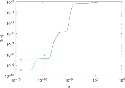
Figure 2. The exact f(t)(−) and its approximation f*(t) with n = m = s = 20, T = 15, and various noise levels added into the measurements data, namely δ = 0.000(− ⋄ −), δ = 0.001(− · −), δ = 0.003(− ○ −), δ = 0.005(− * −) for Example 1.

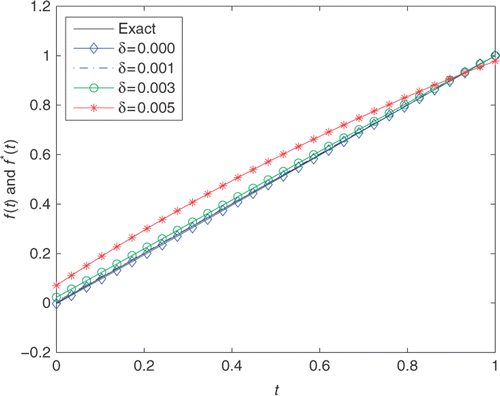
Figure 3. The exact h₂(x)(−) and its approximation with n = m = s = 20, T = 15, and various noise levels added into the measurements data, namely δ = 0.000(− ⋄ −), δ = 0.001(− · −), δ = 0.003(− ○ −), δ = 0.005(− * −) for Example 1.

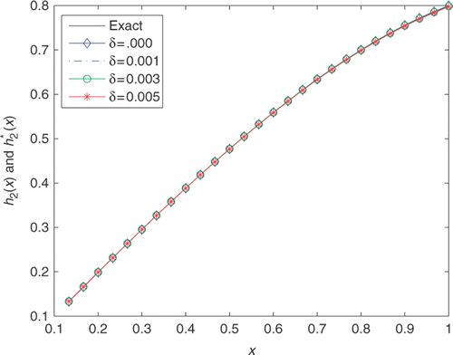
Figure 4. The exact f(t)(−) and its approximation f*(t) with n = m = s = 20, T = 15, and various noise levels added into the measurements data, namely δ = 0.000(− ⋄ −), δ = 0.001(− · −), δ = 0.003(− ○ −), δ = 0.005(− * −) for Example 2.

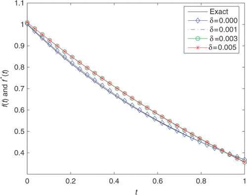
Figure 5. The exact h₂(x)(−) and its approximation with n = m = s = 20, T = 15, and various noise levels added into the measurements data, namely δ = 0.000(− ⋄ −), δ = 0.001(− · −), δ = 0.003(− ○ −), δ = 0.005(− * −) for Example 2.

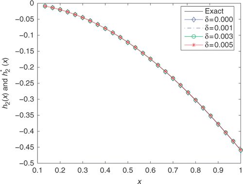
Figure 6. The exact f(t)(−) and its approximation f*(t) with n = m = s = 20, T = 2.5, and various noise levels added into the measurements data, namely δ = 0.000(− ⋄ −), δ = 0.001(− · −), δ = 0.003(− ○ −), δ = 0.005(− * −) for Example 3.

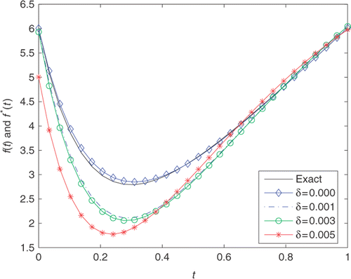
Figure 7. The exact h₂(x)(−) and its approximation with n = m = s = 20, T = 2.5, and various noise levels added into the measurements data, namely δ = 0.000(− ⋄ −), δ = 0.001(− · −), δ = 0.003(− ○ −), δ = 0.005(− * −) for Example 3.

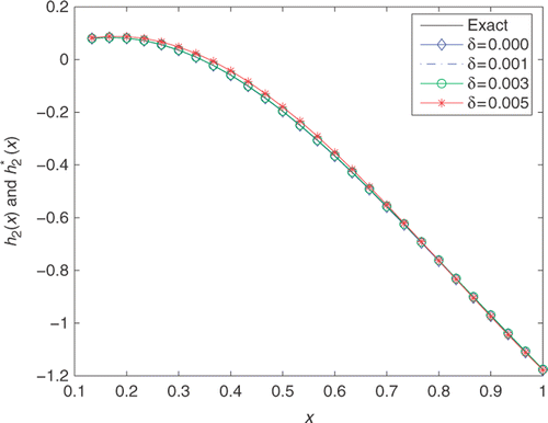
Figure 8. The RRMS(f) with respect to various total numbers of source points with δ = 0.001, T = 2.5, d₁ = d₂ = 0.01 and τ = 0.02 for Example 3.

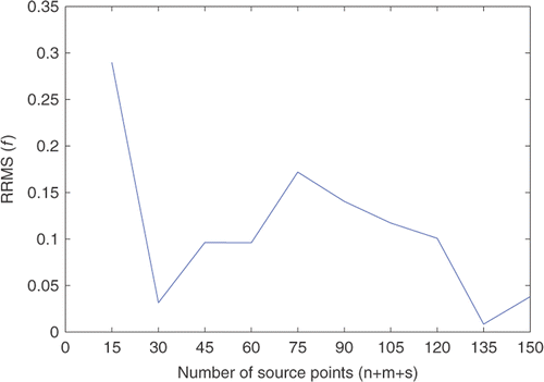
Figure 9. The RRMS(h₂) with respect to various total numbers of source points with δ = 0.001, T = 2.5, d₁ = d₂ = 0.01 and τ = 0.02 for Example 3.

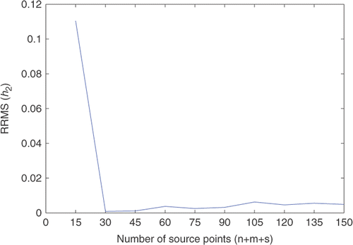
Table 1. The values RMS(f), RRMS(f), RMS(h₂), RRMS(h₂), (δ = 0.001), cond(A) for various values of T for Example 1.

T	RMS(f)	RRMS(f)	RMS(h2)	RRMS(h2)	cond(A)
2.5	0.2351	0.3973	5.1919e−004	9.4642e−004	4.1442e+032
3.5	0.0851	0.1439	0.0012	0.0022	3.3787e+033
10	0.0478	0.0808	6.8315e−004	0.0012	6.0084e+033
20	0.0158	0.0266	2.6395e−004	4.8115e−004	1.8440e+033
100	0.0168	0.0283	0.0035	0.0064	3.4158e+033

Table 2. The values of RRMS(f) for various values of δ and x₀, while T = 15 for Example 2.

x0	δ = 0.01	δ = 0.001	δ = 0.0001
0.1	0.3461	0.0417	0.0038
0.2	0.3048	0.0418	0.0034
0.3	0.2759	0.0416	0.0032
0.4	0.2628	0.0412	0.0038
0.5	0.2607	0.0406	0.0052

Table 3. The values of RRMS(h₂) for various values of δ and x₀, while T = 15 for Example 2.

x0	δ = 0.1	δ = 0.01	δ = 0.001	δ = 0.0001
0.1	0.0939	0.0086	0.0012	2.0372e−004
0.2	0.0774	0.0074	0.0010	2.1433e−004
0.3	0.0669	0.0065	9.1671e−004	2.1848e−004
0.4	0.0708	0.0059	8.4970e−004	2.1559e−004
0.5	0.0619	0.0048	7.5563e−004	2.0424e−004

Table 4. RRMS(f) with respect to various values of d₁, d₂ and τ while x₀ = 0.1, T = 2.5, δ = 0.001 and m = n = s = 20 for Example 3.

d1 d2 τ	0.01	0.02	0.03	0.04	0.05	0.06	0.07	0.08	0.09
0.01	0.0956	0.0956	0.0955	0.0954	0.0953	0.0952	0.0951	0.0950	0.0949
0.02	0.0960	0.0959	0.0958	0.0957	0.0956	0.0955	0.0954	0.0953	0.0951
0.03	0.0964	0.0963	0.0962	0.0961	0.0960	0.0959	0.0958	0.0956	0.0955
0.04	0.0969	0.0968	0.0967	0.0965	0.0964	0.0962	0.0961	0.0960	0.0959
0.05	0.0975	0.0973	0.0972	0.0970	0.0969	0.0968	0.0966	0.0965	0.0964
0.06	0.0980	0.0979	0.0978	0.0976	0.0975	0.0974	0.0972	0.0971	0.0969
0.07	0.0987	0.0986	0.0985	0.0983	0.0982	0.0981	0.0978	0.0977	0.0975
0.08	0.0995	0.0994	0.0993	0.0990	0.0989	0.0987	0.0986	0.0985	0.0983
0.09	0.1004	0.1002	0.1000	0.0999	0.0998	0.0996	0.0995	0.0993	0.0992

Table 5. RRMS(h₂) with respect to various values of d₁, d₂ and τ while x₀ = 0.1, T = 2.5, δ = 0.001 and m = n = s = 20 for Example 3.

d1 d2 τ	0.01	0.02	0.03	0.04	0.05	0.06	0.07	0.08	0.09
0.01	0.0036	0.0036	0.0037	0.0037	0.0035	0.0036	0.0036	0.0036	0.0036
0.02	0.0037	0.0037	0.0036	0.0036	0.0036	0.0037	0.0037	0.0037	0.0036
0.03	0.0037	0.0037	0.0037	0.0037	0.0037	0.0038	0.0038	0.0036	0.0036
0.04	0.0038	0.0038	0.0038	0.0038	0.0038	0.0037	0.0037	0.0037	0.0037
0.05	0.0039	0.0039	0.0039	0.0038	0.0038	0.0038	0.0038	0.0038	0.0038
0.06	0.0039	0.0039	0.0039	0.0039	0.0039	0.0039	0.0039	0.0039	0.0038
0.07	0.0040	0.0040	0.0040	0.0040	0.0040	0.0040	0.0039	0.0039	0.0039
0.08	0.0041	0.0041	0.0041	0.0040	0.0040	0.0040	0.0040	0.0040	0.0040
0.09	0.0042	0.0041	0.0041	0.0041	0.0041	0.0041	0.0041	0.0041	0.0041

6. Conclusion

In this article, we combine the MFS with Tikhonov regularization technique to reconstruct the heat source and partial initial temperature in a heat conduction problem. The numerical examples for various heat sources and initial values are investigated. From the results obtained from the proposed method, we can conclude that the reconstruction of the heat source is much more difficult and sensitive to the noise level than the partial initial temperature, and the more data we input, the better is the accuracy of the numerical solutions. The numerical results show that our proposed method is reasonable, feasible and stable.

Acknowledgements

The author would like to thank the referees and editors for their careful reading and valuable suggestions that improved the quality of our article. The work described in this article was supported by the NNSF of China (10971089).

References

- Hadamard, J, 1923. Lectures on Cauchy's Problem in Linear Partial Differential Equations. New Haven, CT: Yale University Press; 1923.
- Han, H, Ingham, DB, and Yuan, Y, 1995. The boundary element method for the solution of the backward heat conduction equation, J. Comput. Phys. 116 (1995), pp. 292–299.
- Lesnic, D, Elliott, L, and Ingham, D, 1998. An iterative boundary element method for solving the backward heat conduction problem using an elliptic approximation, Inverse Probl. Eng. 13 (1998), pp. 255–279.
- Mera, N, Elliott, L, Ingham, D, and Lesnic, D, 2001. An iterative boundary element method for solving the one dimensional backward heat conduction problem, Int. J. Heat Mass Transf. 44 (2001), pp. 1937–1946.
- Mera, N, Elliott, L, and Ingham, D, 2002. An inversion method with decreasing regularization for the backward heat conduction problem, Numer. Heat Transfer B 42 (2002), pp. 215–230.
- Jourhmane, M, and Mera, N, 2002. An iterative algorithm for the backward heat conduction problem based on variable relaxation factors, Inverse Probl. Eng. 10 (2002), pp. 293–308.
- Kirkup, S, and Wadsworth, M, 2002. Solution of inverse diffusion problems by operator-splitting methods, Appl. Math. Model. 26 (2002), pp. 1003–1018.
- Liu, J, 2002. Numerical solution of forward and backward problem for 2-D heat conduction equation, J. Comput. Appl. Math. 145 (2002), pp. 459–482.
- Iijima, K, 2004. Numerical solution of backward heat conduction problems by a high-order lattice-free finite difference method, J. Chin. Inst. Eng. 27 (2004), pp. 611–620.
- Liu, CS, 2004. Group preserving scheme for backward heat conduction problems, Int. J. Heat Mass Transf. 47 (2004), pp. 2567–2576.
- Mera, NS, 2005. The method of fundamental solutions for the backward heat conduction problem, Inverse Probl. Sci. Eng. 13 (2005), pp. 65–78.
- Liu, CS, Chang, CW, and Chang, JR, 2006. Past cone dynamics and backward group preserving schemes for backward heat conduction problems, CMES Comput. Model. Eng. Sci. 12 (2006), pp. 67–81.
- Chiwiacowsky, LD, and de Campos Velho, HF, 2003. Different approaches for the solution of a backward heat conduction problem, Inverse Probl. Eng. 11 (2003), pp. 471–494.
- Yi, Z, and Murio, DA, 2004. Source term identification in 1-D IHCP, Comput. Math. Appl. 47 (2004), pp. 1921–1933.
- Yi, Z, and Murio, DA, 2004. Identification of source terms in 2-D IHCP, Comput. Math. Appl. 47 (2004), pp. 1517–1533.
- Yamamoto, M, and Zou, J, 2001. Simultaneous reconstruction of the initial temperature and heat radiative coefficient, Inverse Probl. 17 (2001), pp. 1181–1202, Special issue to celebrate Pierre Sabatier's 65th birthday (Montpellier, 2000).
- Li, J, Yamamoto, M, and Zou, J, 2009. Conditional stability and numerical reconstruction of initial temperature, Commun. Pure Appl. Anal. 8 (2009), pp. 361–382.
- Powell, MJD, 1987. "Radial basis functions for multivariable interpolation: A review". In: Mason, JC, and Cox, MG, eds. Algorithms for Approximation (Shrivenham, 1985). New York: Oxford University Press; 1987. pp. 143–167.
- Wu, ZM, 1992. Hermite-Birkhoff interpolation of scattered data by radial basis functions, Approx. Theory Appl. 8 (1992), pp. 1–10.
- Golberg, MA, and Chen, CS, 1999. "The method of fundamental solutions for potential, Helmholtz and diffusion problems". In: Golberg, MA, ed. Boundary Integral Methods: Numerical and Mathematical Aspects. Boston, MA: WIT Press/Computational Mechanics Publications; 1999. pp. 103–176.
- Fairweather, G, and Karageorghis, A, 1998. The method of fundamental solutions for elliptic boundary value problems, Adv. Comput. Math. 9 (1998), pp. 69–95.
- Chen, W, and Hon, YC, 2003. Numerical investigation on convergence of boundary knot method in the analysis of homogeneous Helmholtz, modified Helmholtz, and convection-diffusion problems, Comput. Methods Appl. Mech. Eng. 192 (2003), pp. 1859–1875.
- Chen, W, and Tanaka, M, 2002. A meshless, integration-free, and boundary-only RBF technique, Comput. Math. Appl. 43 (2002), pp. 379–391.
- Kupradze, VD, and Aleksidze, MA, 1964. The method of functional equations for the approximate solution of certain boundary-value problems, Ž. Vyčisl. Mat. Mat. Fiz. 4 (1964), pp. 683–715.
- Mathon, R, and Johnston, RL, 1977. The approximate solution of elliptic boundary-value problems by fundamental solutions, SIAM J. Numer. Anal. 14 (1977), pp. 638–650.
- Kress, R, and Mohsen, A, 1986. On the simulation source technique for exterior problems in acoustics, Math. Methods Appl. Sci. 8 (1986), pp. 585–597.
- Karageorghis, A, and Fairweather, G, 1987. The method of fundamental solutions for the numerical solution of the biharmonic equation, J. Comput. Phys. 69 (1987), pp. 434–459.
- Chen, CS, 1995. The method of fundamental solutions for nonlinear thermal explosions, Commun. Numer. Methods Eng. 11 (1995), pp. 675–681.
- Hon, YC, and Wei, T, 2004. A fundamental solution method for inverse heat conduction problem, Eng. Anal. Boundary Elem. 28 (2004), pp. 489–495.
- Ling, L, Hon, YC, and Yamamoto, M, 2005. Inverse source identification for Poisson equation, Inverse Probl. Sci. Eng. 13 (2005), pp. 433–447.
- Ling, L, Yamamoto, M, Hon, YC, and Takeuchi, T, 2006. Identification of source locations in two-dimensional heat equations, Inverse Probl. 22 (2006), pp. 1289–1305.
- Yan, L, Fu, CL, and Yang, FL, 2008. A fundamental solution method for inverse heat conduction problem, Eng. Anal. Boundary Elem. 28 (2008), pp. 489–495.
- Yan, L, Yang, FL, and Fu, CL, 2009. A meshless method for solving an inverse spacewise-dependent heat source problem, J. Comput. Phys. 228 (2009), pp. 123–136.
- Shidfar, A, Darooghehgimofrad, Z, and Garshasbi, M, 2009. Note on using radial basis functions and Tikhonov regularization method to solve an inverse heat conduction problem, Eng. Anal. Boundary Elem. 33 (2009), pp. 1236–1238.
- Tikhonov, AN, and Arsenin, VY, Solutions of Ill-posed Problems, Scripta Series in Mathematics. Washington, DC: V. H. Winston & Sons, John Wiley & Sons, New York, 1977 (Translated from the Russian, Preface by translation editor F. John.).
- Isakov, V, 1990. "Inverse Source Problems". In: Mathematical Surveys and Monographs. Vol. 34. Providence, RI: American Mathematical Society; 1990.
- Hon, YC, and Wei, T, 2005. The method of fundamental solution for solving multidimensional inverse heat conduction problems, CMES Comput. Model. Eng. Sci. 7 (2005), pp. 119–132.
- Hansen, PC, 1998. Rank-deficient and Discrete Ill-posed Problems: Numerical Aspects of Linear Inversion. Philadelphia, PA: SIAM Monographs on Mathematical Modeling and Computation, Society for Industrial and Applied Mathematics (SIAM); 1998.
- Wahba, G, and Wendelberger, J, 1980. Some new mathematical methods for variational objective analysis using splines and cross validation, Monthly Weather Rev. 108 (1980), pp. 1122–1143.
- Hansen, PC, 1994. Regularization tools: A Matlab package for analysis and solution of discrete ill-posed problems, Numer. Algorithms 6 (1994), pp. 1–35.