Comparative analysis of inverse coefficient problems for parabolic equations. Part I: adjoint problem approach

Abstract

This article presents a mathematical and computational analysis of the adjoint problem approach for parabolic inverse coefficient (or inverse heat conduction) problems based on boundary measured data. In Part I the mathematical analysis is given for three classes of typical inverse coefficient problems with various Neumann or/and Dirichlet types of measured output data. Although all three types of considered inverse coefficient problems are severely ill-posed, comparative numerical analysis show that the ill-posedness depends also on where the Neumann and Dirichlet conditions are given: in the direct problem or as an output data. For all these types of inverse problems the integral identities relating solutions of direct problems and appropriate adjoint problems solutions are derived. These integral identities permit proof of monotonicity, Lipschitz continuity, and hence invertibility of the corresponding input–output mappings. Based on these results solvability of all three types of inverse coefficient problems are proved. The degree of ill-posedness of inverse problems is demonstrated on numerical test examples.

Keywords:

• adjoint problem approach
• coefficient identification
• input–output mappings
• monotonicity
• Lipschitz continuity
• ill-posedness

AMS Subject Classifications:

• 35R30
• 35K05
• 65N50

1. Introduction

Consider the following initial boundary value problem: (1) where Ω_T = {(x, t) ∈ ℝ² : 0 < x < 1, 0 < t ≤ T}. Let us define the class of admissible coefficients as follows: 𝒦 ≔ {k(x) ∈ L_∞[0, 1] : 0 < c₀ ≤ k(x) ≤ c₁}. It is assumed that the function ν₀(t) > 0 for all t ∈ (0, T), belongs to H¹[0, T ] and satisfies the consistency condition: ν₀(0) = 0. These conditions will be defined below as the conditions (C1). Under these conditions the initial boundary value problem (1) has a unique solution in (see, e.g. 1).

Consider the inverse problem of determining the unknown coefficient k = k(x) from the following measured output (flux) data given at the boundary: (2) where u = u(x, t; k) is the solution of the parabolic problem (1) for a given k(x) ∈ 𝒦. The functions f_i(t) are defined to be the Neumann-type measured output data, according to 2–9. In this context the parabolic problem (1) will be referred to as a direct (forward) problem, with the Dirichlet-type input data ν₀(t). It is assumed that the outputs f_i(t) belong to H⁰[0, T ], and satisfy the consistency conditions: f₀(0) = f₁(0) = 0. These conditions will be defined below as the conditions (C2). The inverse coefficient problem (1)–(2) will be referred to as ICP1.

Let us consider now the inverse problem of determining the unknown coefficient k(x) ∈ 𝒦 in the parabolic problem (with mixed boundary conditions) (3) from the following Dirichlet or/and Neumann-type measured output data (4) Here u(x, t; k) is the solution of the direct problem (3) for a given k(x) ∈ 𝒦. It is assumed that the input data f₀(t) and the output data ν₀(t) satisfy the consistency conditions: f₀(0) = ν₀(0) = 0. The inverse coefficient problem (3)–(4) will be referred to as ICP2.

Finally, consider the inverse problem of determining the unknown coefficient k(x) ∈ 𝒦 in the parabolic problem (with Neumann boundary conditions) (5) from the following Dirichlet-type measured output data (6) The inverse coefficient problem (5)–(6) will be referred to as ICP3.

Let us analyse the problem ICP1. Let u = u(x, t; k) be the unique solution of the direct problem (1) for a given coefficient k(x) ∈ 𝒦. Then the left flux (−k(x)u_x(x, t; k))_x=0 represents the output data, corresponding to the given coefficient k(x). According to the additional condition (2), k(x) ∈ 𝒦 is the solution of the problem ICP1 if the identity (−k(x)u_x(x, t; k))_x=0 ≡ f₀(t), ∀t ∈ (0, T ] between the output data and measured output data holds. Hence, introducing the input–output (or coefficient-data) mapping Φ₀[·] : 𝒦 ↦ ℱ ⊂ H⁰(0, T), where Φ₀[k](t) ≔ (−k(x)u_x(x, t; k))_x=0, one can formulate the inverse problem as the following operator equation: (7) Therefore, the problem ICP1 with the given measured output data f₀(t) can be reduced to the solution of the nonlinear equation (7) or to inverting the input–output mapping Φ₀[·] : 𝒦 ↦ ℱ.

Similar input–output mappings can be introduced for ICP2 and ICP3. This approach has been introduced in 2–4, for nonlinear parabolic equations, and in 5–8, for linear parabolic equations.

Since any output measured data can only be given with some error, the most common approach for identifying the unknown coefficient is based on introducing the error (or auxiliary) functional (8) and reformulating the inverse problem as a minimization problem for the functional J₁(k). The methods based on this approach are defined as quasi-solution methods, according to 9, or the output least squares (OLS) 10–13. Typical difficulties arising in this approach are lack of uniqueness, convergence to false minima and numerical instability.

An alternative to coefficient identification by OLS methods is the equation error method 14–17. Here the measured output data is used as input to the differential equation in the direct problem. Then this problem is reformulated as an equation with respect to the unknown coefficient k = k(x). As a consequence, this equation expresses a direct relationship between the values of the unknown coefficient and measured data. This relationship is problem dependent and frequently quite complicated. For this reason it is not easy to find out from its properties the input–output mappings in equation error methods.

The adjoint problem approach, proposed in 2–8 for coefficient and source identification problems, related to nonlinear parabolic equations, is based on appropriate adjoint problem to direct problem. The first distinguishable feature of the approach is that, for each direct problem, there exists a unique adjoint problem with arbitrary boundary data in the form of Dirichlet or Neumann condition(s). Further, for each direct problem there exists an integral relationship between the solutions of these problems. These relationships act as an effective computational tool for the numerical solution of inverse coefficient and source problems. The second distinguishable feature of the adjoint problem approach is that by choosing the above-mentioned arbitrary boundary data monotonicity and invertibility of the input–output mappings, solvability of the inverse problems can be proved. Moreover, use of measured output data in adjoint problems allows one to obtain an explicit formula for the gradient of cost functionals for each inverse problem.

This article presents a mathematical analysis of the adjoint problem approach for the above-formulated typical inverse coefficient problems with various Neumann or/and Dirichlet-type measured output data. For each type of these problems, corresponding integral relationships, are derived. Using these relationships, solvability of each inverse problem is proved. Although all types of inverse coefficient problems are severely ill-posed, it is shown that this ill-posedness also depends on where the Neumann and Dirichlet boundary conditions are given: in the direct problem or as a measured output data. Depending on the type of boundary conditions, three classes of inverse problems are discussed in this study. In the first class of inverse problems the Dirichlet boundary conditions u(0, t) = ν₀(t), u(1, t) = 0 are imposed in the direct problem, and the Neumann condition f₀(t) ≔ −k(0)u_x(0, t) is defined to be an additional condition for the determination of the unknown coefficient k(x). In the second class of inverse problems the Neumann and Dirichlet boundary conditions −k(0)u_x(0, t) = f₀(t), u(1, t) = 0 are imposed in the direct problem, and the Dirichlet boundary condition ν₀(t) ≔ u(0, t) is defined as an additional condition for determination of the unknown coefficient k(x). In the third class of inverse problems the Neumann conditions −k(0)u_x(0, t) = f₀(t), u_x(0, t) = 0 are imposed in the direct problem, and the Dirichlet boundary condition ν₀(t) ≔ u(0, t) is defined to be as a measured output data. For all these inverse problems, integral identities relating the solution of direct problems and appropriate adjoint problems are derived. Based on these identities, monotonicity and Lipschitz continuity of the input–output mappings are proved. These results agree with the proof of the solvability of the considered coefficient identification problems.

This article is organized as follows. In Section 2, an integral identity relating changes in the diffusion coefficient to changes of measured output data is derived for ICP1. This identity, with the deduced properties of the direct problem solution, allow proof of the monotonicity of the input–output mappings. Then the Lipschitz continuity of these mappings is proved. These results permit one to prove the solvability of ICP1. In Section 3, all these results are extended to the other inverse problems. Computational experiments related to the degree of ill-posedness of inverse coefficient problems are presented in Section 4. Conclusions are presented in Section 5.

2. An analysis of ICP1

The result below is crucial in the solvability of ICP1.

Lemma 2.1

Let conditions (C1) and (C2) hold. Assume that u₁(x, t) = u(x, t; k_i), i = 1, 2, are solutions of the direct problem (1), corresponding to the admissible coefficients k_i(x) ∈ 𝒦. Denote by , (i = 1, 2) the corresponding outputs. Then for each τ ∈ (0, T ] the following integral identity holds: (9) between the solution of the direct problem (1) and the corresponding adjoint problem (10) where , , Δk(x) = k₁(x) − k₂(x) and p(t), q(t) ∈ C(0, T ] are arbitrary data.

Proof

The function Δu(x, t) = u₁(x, t) − u₂(x, t) satisfies the parabolic problem Multiplying both sides of the above partial differential equation by the arbitrary function ϕ(x, t) and integrating on Ω_τ by parts, one obtains (11) Assume that the function ϕ(x, t) satisfies the backward parabolic problem (10). Then the sum of the first and third left-hand side integrals in (11) is zero due to Equation (10). Further, by the homogeneous initial (u(x, 0) = 0) and final (ϕ(x, τ) = 0) conditions, and the homogeneous boundary conditions Δu(0, t) = Δu(1, t) = 0, the second and fifth left-hand side integrals are also zero. Hence we have (12) We have Using these with the boundary conditions ϕ(0, t) = p(t), ϕ(1, t) = q(t) in the integral identity (12), we obtain the required relationship (9).▪

Consider some special cases. First, assume that q(t) ≡ 0 in the adjoint problem (10): (13) Then the integral relationship (9) has the form (14) This integral relationship (as well as the adjoint problem (13)) corresponds to ICP1 with the Neumann-type measured output data f₀(t), given by (2).

Now assuming p(t) ≡ 0 in the adjoint problem (10) we get (15) Then the integral relationship (9) has the form (16) The integral relationship (16) (as well as the adjoint problem (15)) corresponds to the problem (ICP1) with the Neumann-type measured output data f₁(t), given by (2).

The integral relationship (9) (as well as the adjoint problem (10)) corresponds to ICP1 with two Neumann-type measured output data f₀(t) and f₁(t), given by (2).

The next result shows behaviour of the solution of ICP1, in particular the behaviour of the output data at the boundary.

Lemma 2.2

Let conditions (C1) and (C2) hold, and u(x, t; k) be the solution of the direct problem (1), corresponding to the admissible coefficient k(x) ∈ 𝒦 ∩ C¹[0, 1]. Then u_x(x, t; k) ≤ 0, ∀(x, t) ∈ Ω_T.

Proof

Multiply both sides of the heat equation in (1) by the arbitrary test function ψ_x(x, t), integrate on Ω_τ ≔ (0, 1) × (0, τ), τ ∈ (0, T ] and apply integration by parts: Assume that the function ψ(x, t) is the solution of the following backward parabolic problem: with the arbitrary continuous source function which will be defined below. The first and second right-hand side integrals in the above identity are zero due to the homogeneous initial (u(x, 0) = 0), final (ψ(x, τ) = 0) and boundary conditions. Taking into account the boundary condition ψ_x(1, t) = 0 in the third right-hand side integral, we obtain (17) We require that the function F(x, t) is positive in Ω_τ, i.e. F(x, t) > 0. Since and k(x) ∈ C¹[0, 1], the solution ψ(x, t) of the above backward parabolic problem belongs to . Then applying the maximum principle 18 to the backward parabolic problem, we conclude that ψ(x, t) < 0 in Ω_τ. This, in particular means that ψ_x(0, t) ≤ 0, since On the other hand, the max–min principle applied to the direct problem (1) with the positivity of the Dirichlet input data ν₀(t) > 0 implies ν₀(t) > u(x, t) > 0, ∀(x, t) ∈ Ω_T, which means u_x(0, t) ≤ 0. Thus the right-hand side integral in (17) is negative which means that for all F(x, t) > 0, Due to the fact that the function F(x, t) > 0 is arbitrary and τ ∈ (0, T ], we have the proof. ▪

Corollary 2.1

The sign of input data in the direct problem (1) can define the sign of output data, i.e. if ν₀(t) > 0, then f₀(t) = −k(0)u_x(0, t; k) ≥ 0 and f₁(t) = −k(1)u_x(1, t; k) ≥ 0.

Let us analyse now the monotonicity of input–output mapping given by (7).

Lemma 2.3

Let conditions of Lemma 2.2 hold. If the admissible coefficients k₁(x), k₂(x) ∈ 𝒦 satisfy the condition k₁(x) > k₂(x), ∀x ∈ [0, 1], then the input–output mapping Φ₀[k](t) ≔ (−k(x)u_x(x, t; k))_x=0 has the following property: (18)

Proof

To prove this lemma we will use the integral relationship (14), assuming that the arbitrary function p(t) in the adjoint problem (13) is positive: p(t) > 0, ∀t ∈ (0, T). For the solution u₂(x, t) = u(x, t; k₂) of the direct problem (1) we conclude u_2x(x, t) ≤ 0, according to Lemma 2.2. Due to the positivity of function p(t), the same conclusion is valid for the solution ϕ(x, t) of the adjoint problem (13): ϕ(x, t) > 0, ϕ_x(x, t) ≤ 0. Then from the integral relationship (14) we conclude that where Δf₀(t) = Φ₀[k₁](t) − Φ₀[k₂](t). This implies (18).▪

This lemma asserts that the input–output mapping Φ₀[·] : K ↦ ℱ defined by (7) is a monotone mapping. Physical interpretation of this property is that in the case of the same temperature u(0, t) = ν₀(t) > 0 at the left end of two bars, higher thermal conductivity k(x) will generate higher left flux.

Similarly, we may introduce the input–output mapping Φ₁[k](t) ≔ (−k(x)u_x(x, t; k))_x=1, and prove the following result.

Lemma 2.4

Let the conditions of Lemma 2.2 hold, and coefficients k₁(x), k₂(x) ∈ 𝒦 satisfy the condition k₁(x) > k₂(x), ∀x ∈ [0, 1]. Then the input–output mapping Φ₁[k](t) ≔ (−k(x)u_x(x, t; k))_x=1 is an antitone one, i.e. (19)

The following lemma shows that the input–output mappings Φ₀[k](t) and Φ₁[k](t) are both injective.

Lemma 2.5

Let conditions of Lemma 2.2 hold and k₁(x), k₂(x) ∈ 𝒦. Then

a.	Φ0[k1](t) = Φ0[k2](t) implies k1(x) = k2(x), a.e. x ∈ [0, 1];
b.	Φ1[k1](t) = Φ1[k2](t) implies k1(x) = k2(x), a.e. x ∈ [0, 1].

Proof

The proof follows directly from the integral identities (14) and (16). Indeed, since , i = 1, 2, and substituting in the right-hand side integral of (14) , we obtain (20) If u₂(x, t) = u(x, t; k₂) is the solution of the direct problem (1) for the given k₂(x) ∈ 𝒦, then we conclude u_2x(x, t) ≤ 0, according to Lemma 2.2. As in the proof of Lemma 2.2, for the positive control function p(t) in (13), the same conclusion is valid for the solution ϕ(x, t) of the adjoint problem (13): ϕ_x(x, t) ≤ 0. Due to the fact that the control function p(t) in (13) is arbitrary, we may take p(t) < 0 and conclude that ϕ_x(x, t) ≥ 0. Taking this into account in (20), we conclude that Δk(x) ≡ 0, a.e. x ∈ [0, 1], which completes the first part of the lemma.

The second part of the lemma can be proved similarly.▪

Using the above results, now we can prove the Lipschitz continuity of the input–output mappings corresponding to ICP1.

Theorem 2.1

If conditions of Lemma 2.2 hold, then input–output mappings Φ₀[·] : 𝒦 ↦ ℱ and Φ₁[·] : 𝒦 ↦ ℱ are Lipschitz continuous mappings:

i.
ii.

where and are the Lipschitz constants, ϕ₀(x, t) = ϕ(x, t; p, 0), ϕ₁(x, t) = ϕ(x, t; 0, q) are solutions of the adjoint problems (13) and (15), respectively, and p and q are defined below.

Proof

Let us define , i = 1, 2, and choose the function p(t) in the adjoint problem (13) as follows: Substituting this into (14) and taking τ = T, we get Applying the Cauchy inequality to the right-hand side integral, we obtain (i).

The second part of the theorem can be proved by the same way, taking in the adjoint problem (15) where , i = 1, 2.▪

Having the monotonicity and Lipschitz continuity of the mappings Φ₀[·] : 𝒦 ↦ ℱ, and Φ₁[·] : 𝒦 ↦ ℱ, we obtain the following theorem.

Theorem 2.2

Let conditions of Lemma 2.2 hold. Then the ICP1 with the flux data f₀(t) (or f₁(t)), given by (2), has a unique solution.

3. An analysis of ICP2 and ICP3

Now let us extend the above results to ICP2.

Lemma 3.1

Let conditions (C1) and (C2) hold. Assume that u_i(x, t) = u(x, t; k_i), i = 1, 2, are solutions of the direct problem (3), corresponding to the admissible coefficients k_i(x) ∈ 𝒦. Denote by , the corresponding outputs, and let Δk(x) = k₁(x) − k₂(x). Then for each τ ∈ (0, T ] the following integral identity holds: (21) between the solution of the direct problem (3) and the corresponding adjoint problem (22) where , and p(t), q(t) ∈ C(0, T ] are arbitrary data.

Proof

We use the proof scheme of Lemma 2.1. The function Δu(x, t) = u₁(x, t) − u₂(x, t) satisfies the parabolic problem (23) Multiplying both sides of the above partial differential equation by the arbitrary function ϕ(x, t) and integrating by parts on Ω_τ, we obtain the integral identity (11). Using the initial (Δu(x, 0) = 0), final (ϕ(x, τ) = 0) and boundary conditions in problems (22) and (23), then taking into account that the function ϕ(x, t) satisfies the backward parabolic equation (22), we obtain the integral relationship (21).▪

The backward parabolic problem (22) is defined to be the adjoint problem corresponding to ICP2 with two, Dirichlet ν₀(t) and Neumann f₁(t) measured output data, given by (4).

Consider the special cases when only one measured output data is given. First, assume that q(t) ≡ 0 in the adjoint problem (22): (24) Then the integral relationship (21) has the form (25) This integral relationship (as well as the adjoint problem (24)) corresponds to the problem ICP2 with the Dirichlet-type measured output data ν₀(t), given by (4).

Now assuming p(t) ≡ 0 in the adjoint problem (22), we get (26) Then the integral relationship (21) has the form (27) The integral relationship (27) (as well as the adjoint problem (26)) corresponds to the problem ICP2 with the Neumann-type measured output data f₁(t), given by (4).

The next result shows behaviour of the solution of the problem ICP2, in particular the behaviour of the output data at the boundary.

Lemma 3.2

Let conditions (C1) and (C2) hold, and u(x, t; k) be the solution of the direct problem (3), corresponding to the admissible coefficient k(x) ∈ 𝒦 ∩ C¹[0, 1]. Assume, in addition, that f₀(t) ∈ C[0, 1]. If f₀(t) > 0, then u_x(x, t; k) ≤ 0, ∀(x, t) ∈ Ω_T.

Proof

As in the proof of Lemma 2.2 we obtain, compare (17), (28) Requiring the positiveness of the function F(x, t) in Ω_τ, as in the proof of Lemma 2.2, we conclude that ψ_x(0, t) ≤ 0. Hence the right-hand side integral in (28) is negative which means that for all F(x, t) > 0 Due to the fact that the function F(x, t) > 0 is arbitrary and τ ∈ (0, T ], we have the proof. ▪

Let us now introduce the input–output mapping Ψ₀[·] : 𝒦 ↦ 𝒩₀ by Ψ₀[k](t) ≔ u(0, t; k). Then in the case of the left (ν₀(t)) and right (f₁(t)) output measured data, the ICP2 can be reformulated, respectively, as follows: (29) The monotonicity of these mappings is given by the following lemma.

Lemma 3.3

Let conditions of Lemma 3.2 hold. Assume that u(x, t; k_i), i = 1, 2, is the solution of the direct problem (3), corresponding to the admissible coefficients k_i(x) ∈ 𝒦. If k₁(x) > k₂(x), ∀x ∈ [0, 1], then the operators in (29) are antitone, i.e.

i.	Ψ0[k1](t) ≤ Ψ0[k2](t), ∀t ∈ [0, T ];
ii.	Φ1[k1](t) ≤ Φ1[k2](t), ∀t ∈ [0, T ].

Proof

To prove (i) we will use the integral relationship (25), assuming that the arbitrary function p(t) in the adjoint problem (24) is positive: p(t) > 0, ∀t ∈ (0, T). For the solution u₂(x, t) = u(x, t; k₂) of the direct problem (3) we conclude u_2x(x, t) ≤ 0, according to Lemma 3.2. Due to positiveness of function p(t), the same conclusion is valid for the solution ϕ(x, t) of the adjoint problem (24): ϕ_x(x, t) ≤ 0. Then the integral relationship (25), with Δν₀(t) = Ψ₀[k₁](t) − Ψ₀[k₂](t), implies This implies (i). The second part (ii) can be obtained by the same way.▪

Using the proof of Lemma 2.5, we can also prove that the above defined input–output mappings Ψ₀[k](t) and Φ₁[k](t) are both injective.

Lemma 3.4

Let conditions of Lemma 3.2 hold and k₁(x), k₂(x) ∈ 𝒦. Then

a.	Ψ0[k1](t) = Ψ0[k2](t) implies k1(x) = k2(x), a.e. x ∈ [0, 1];
b.	Φ1[k1](t) = Φ1[k2](t) implies k1(x) = k2(x), a.e. x ∈ [0, 1].

The following theorem shows that the above-defined input–output mappings are Lipschitz continuous.

Theorem 3.1

If conditions of Lemma 3.2 hold, then input–output mappings Ψ₀[·] : 𝒦 ↦ 𝒩₀ and Φ₁[·] : 𝒦 ↦ ℱ, corresponding to ICP2 are Lipschitz continuous:

i.
ii.

where and are the Lipschitz constants, ϕ₀(x, t) = ϕ(x, t; p, 0), ϕ₁(x, t) = ϕ(x, t; 0, q) are solutions of the adjoint problems (24) and (26), respectively, p is defined below and q is defined as in Theorem 2.1.

Proof

We define , i = 1, 2, and choose the function p(t) in the adjoint problem (24) as follows: Substituting this into (25) and assuming that τ = T, we get Applying the Cauchy inequality to the right-hand side integral, we obtain (i).

The second part of the theorem can be proved in the same way.▪

The monotonicity and Lipschitz continuity of the input–output mappings allow the formulation of the following solvability theorem.

Theorem 3.2

Let conditions of Lemma 3.2 hold. Then the ICP2 with Dirichlet (or Neumann) data, given by (4) has a unique solution.

Although an analysis of ICP3 has been given in 5, for completeness of the study we will derive here the result (Lemma 2, 5) related to the relationship, i.e. integral identity, between the direct problem (5) and the corresponding adjoint problem.

Lemma 3.5

Let conditions (C1) and (C2) hold. Assume that u_i(x, t) = u(x, t; k_i), i = 1, 2, are solutions of the direct problem (5), corresponding to the admissible coefficients k_i(x) ∈ 𝒦. Denote by , the corresponding outputs, and let Δk(x) = k₁(x) − k₂(x). Then for each τ ∈ (0, T ] the following integral identity holds: (30) between the solution of the direct problem (5) and the corresponding adjoint problem (31) where , and p(t), q(t) ∈ C(0, T ] are arbitrary data.

Assuming q(t) ≡ 0 in (31), we get (32) Then the integral relationship (30) has the form (33) This integral relationship with the adjoint problem (32) corresponds to ICP3 with the Dirichlet-type measured output data ν₀(t), given by (6).

Now assuming p(t) ≡ 0 in the adjoint problem (31), we obtain (34) Then the integral relationship (30) has the form (35) The integral relationship (35) (as well as the adjoint problem (34)) corresponds to ICP3 with the Dirichlet-type measured output data ν₁(t), given by (6). Due to the presence of the both output data ν₀(t) and ν₁(t), the integral relationship (30) with the adjoint problem (31) corresponds to ICP3 with two Dirichlet-type measured output data ν₀(t) and ν₁(t) given by (6).

4. Comparative numerical analysis of ill-posedness of the inverse coefficient problems

Although all three inverse coefficient problems are severely ill-posed, in the sense that small changes in the output data does not correspond to small changes in the coefficient k(x), this ill-posedness also depends on where the Neumann and Dirichlet conditions are given: in the direct problem or as an output data. To illustrate this situation the synthetic output data is generated using numerical solutions of direct problems (1), (3) and (5), corresponding to ICP1, ICP2 and ICP3, respectively. The finite-difference analogue of the direct problem (1) is the following discrete problem: (36) This implicit difference scheme has the order of approximation when the solution u(x, t) of the direct problem belongs to the class C^4,2(Ω_T) 19.

To generate the discrete analogue of the synthetic output data f₀(t)[k] ≔ −k(0)u_x(0, t; k), the discrete problem (36) is solved on the uniform grid ω_h ≔ {(x_i, t_j) : x₀ = 0, x_i+1 = x_i + h_x, t₀ = 0, t_j+1 = t_j + h_t}, with the grid steps h_x = 1/N, h_t = 1/M, for a coefficient k(x) and Dirichlet data ν₀(t). The output data is calculated from the following difference scheme: which is obtained from the above implicit difference scheme.

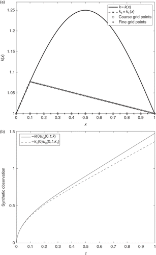
In the first series of computational experiments, the discrete problem (36) was solved for the coefficient k(x) = 1 + 0.25 sin(πx), and for its piecewise linear approximation k₁(x), with k₁(0) = k(0) = 1 and k₁(1) = k(1) = 1, by using Lagrange-type basic functions on a coarser mesh (Figure 1a). In both cases the Dirichlet-type input data was assumed to be ν₀(t) = t. The obtained approximate values and of the output data f₀(t)[k] ≔ −k(0)u_x(0, t; k) and f₀(t)[k₁] ≔ −k(0)u_x(0, t; k₁) are plotted in Figure 1(b). It is seen from these figures that although the coefficients k(x) and k₁(x) are quite different, the corresponding output data and are close enough. Specifically, the absolute sup-norm error in the output data is ϵ₁[ f₀] = 0.11, while the absolute sup-norm error in the coefficients is ϵ₁[k] = 0.22.

Figure 1. Ill-posed nature of ICP1: k(x) = 1 + 0.25 sin(πx), ν₀(t) = t.

In the case of ICP2, one needs to replace the first Dirichlet condition in the discrete problem (36) by the Neumann condition: (37) The discrete analogue of the synthetic output data ν(t)[k] ≔ u(0, t; k) is calculated from the numerical solution of problem (37).

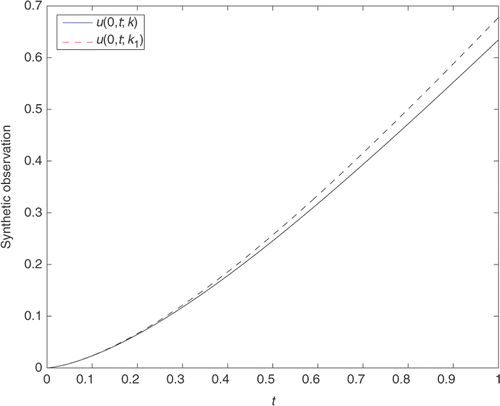
To see the degree of ill-posedness of ICP2, a second series of computational experiments were performed for the discrete problem (37). To make the experiment comparable with the previous one, the same coefficient k(x) = 1 + 0.25 sin(πx), with its same piecewise linear approximation k₁(x) was taken (Figure 1a). In both cases the Neumann-type input data was assumed to be f₀(t) = t. The obtained approximate values and of the output data ν₀(t)[k] ≔ u(0, t; k) and ν₀(t)[k₁] ≔ u(0, t; k₁) are plotted in Figure 2. For the same absolute sup-norm error ϵ₁[k] = 0.22 in the coefficients, the absolute sup-norm error in the Dirichlet-type output data is ϵ₂[ν₀] = 0.043, which is less than ϵ₁[ f₀] = 0.11 obtained for ICP1.

Figure 2. Ill-posed nature of ICP2: k(x) = 1 + 0.25 sin(πx), f₀(t) = t.

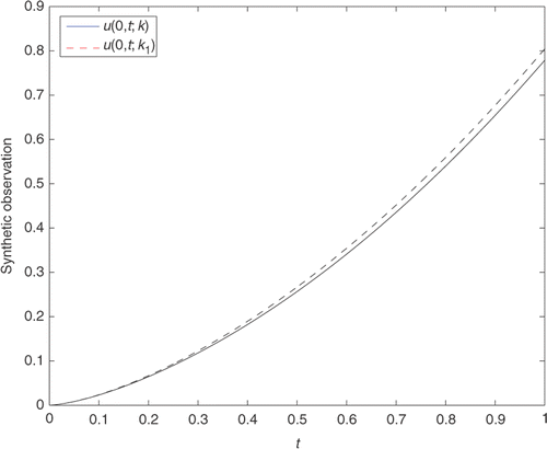
In the case of ICP3, one needs to replace the second Dirichlet condition in the discrete problem (37) by the Neumann condition (38) The discrete analogue of the synthetic output data here is the same as in ICP2. The above coefficients k(x) and k₁(x) and also the same Neumann-type input data f₀(t) = t was taken in the computational experiments. The outputs from the numerical solution of the discrete problem (38) are plotted in Figure 3. The figure shows that for the same absolute sup-norm error ϵ₁[k] = ϵ₃[k] = 0.22 in the coefficients the absolute sup-norm error in the Dirichlet output data is ϵ₂[ν₀] = 0.026, which is less than the error 0.043 obtained for ICP2.

Figure 3. Ill-posed nature of ICP3: k(x) = 1 + 0.25 sin(πx), f₀(t) = t.

Note that in all the computational experiments the grid parameters N and M were taken to be N = 100 and M = 200, and any further increase of these parameters did not change the obtained results significantly.

5. Conclusions

The aim of this article was to demonstrate an implementation of the adjoint problem approach in the mathematical analysis of coefficient identification problems for linear parabolic equations. The presented approach permits one to prove monotonicity, Lipschitz continuity, and hence invertibility of input–output mappings corresponding to each type of inverse problem. Note that such types of results cannot be obtained either from the output least-squares approach or from equation error techniques. The presented computational results show that ICP1 is less ill-posed than ICP2 and ICP3. This, in particular means that, one can suitably define the Dirichlet data as an input data, and the Neumann data as a measured output data. The feasibility of the implementation of the integral identities relating to each inverse coefficient problem will be discussed in Part II.

Finally, it should be noted that the above-presented results have no obvious extensions to higher dimensions. However, in the case of a rectangular domain Ω ≔ (0, l_x) × (0, l_y), extension of Theorem 2.2, under some additional conditions, is possible. These studies are in progress.

Acknowledgements

This research was supported by the Scientific and Technological Research Council of Turkey (TUBITAK) through the project No. 108T332. The work of A. Hasanov was supported by the International Research Program of L.N. Gumilev Eurasian National University, Astana, Kazakhstan. The authors would like to thank to the referees whose comments and suggestions substantially improved the revision of this article.

References

- Ladyzhenskaya, OA, 1985. Boundary Value Problems in Mathematical Physics. New York: Springer Verlag; 1985.
- DuChateau, P, 1995. Monotonicity and invertibility of coefficient-to-data mappings for parabolic inverse problems, SIAM J. Math. Anal. 26 (1995), pp. 1473–1487.
- DuChateau, P, 1996. "Introduction to inverse problems in partial differential equations for engineers, physicists and mathematicians". In: Gottlieb, J, and DuChateau, P, eds. Parameter Identification and Inverse Problems in Hydrology, Geology and Ecology. Dordrecht: Kluwer Academic Publishers; 1996. pp. 3–38.
- DuChateau, P, Thelwell, R, and Butters, G, 2004. Analysis of an adjoint problem approach to the identification of an unknown diffusion coefficient, Inverse Probl. 20 (2004), pp. 601–625.
- Hasanov, A, DuChateau, P, and Pektas, B, 2006. An adjoint problem approach and coarse-fine mesh method for identification of the diffusion coefficient in a linear parabolic equation, J. Inverse Ill-Posed Probl. 14 (5) (2006), pp. 435–463.
- Hasanov, A, 2007. Simultaneous determination of source terms in a linear parabolic problem from the final overdetermination: Weak solution approach, J. Math. Anal. Appl. 330 (2007), pp. 766–779.
- Hasanov, A, Demir, A, and Erdem, A, 2007. Monotonicity of input–output mappings in inverse coefficient and source problems for parabolic equations, J. Math. Anal. Appl. 335 (2007), pp. 1434–1451.
- Kabanikhin, SI, Hasanov, A, and Penenko, AV, 2008. A gradient descent method for solving an inverse coefficient heat conduction problem, Numerical Anal. Appl. 1 (1) (2008), pp. 34–45.
- Ivanov, VK, Vasin, VV, and Tanana, VP, 1978. Theory of Linear Ill-Posed Problems and Its Applications. Nauka, Moscow. 1978.
- Chavent, G, and Lemonnier, P, 1974. Identification de la non-linearite d'une equation parabolique quasilinearie, Appl. Math. Optim. 1 (1974), pp. 121–162.
- Jarny, Y, Ozisik, MN, and Bardon, JP, 1991. A general optimization method using adjoint equation for solving multidimensional inverse heat conduction, Int. J. Heat Mass Transfer 34 (1991), pp. 2911–2918.
- Knabner, P, and Bitterlilich, S, 2002. An efficient method for solving an inverse problem for the Richards equation, J. Comput. Appl. Math. 147 (2002), pp. 153–173.
- Nabakov, R, 1996. "An inverse problem for porous medium equation". In: Gottlieb, J, and DuChateau, P, eds. Parameter Identification and Inverse Problems in Hydrology, Geology and Ecology. Dordrecht: Kluwer Academic Publishers; 1996. pp. 155–163.
- Cannon, JR, and DuChateau, P, 1987. Design of an experiment for the determination of a coefficient in a nonlinear diffusion equation, Int. J. Eng. Sci. 25 (1987), pp. 1067–1078.
- Hanke, M, and Scherzer, O, 1999. Error analysis of an equation error method for the identification of the diffusion coefficient in a quasilinear parabolic differential equation, SIAM J. Appl. Math. 59 (1999), pp. 1012–1027.
- Reeve, DE, and Spivack, M, 1999. Recovery of a variable coefficient in a coastal evolution equation, J. Comput. Phys. 151 (1999), pp. 585–596.
- Richter, GR, 1981. Numerical identification of a spatially varying diffusion coefficient, Math. Comput. 36 (1981), pp. 375–386.
- Protter, MH, and Weinberger, HE, 1967. Maximum Principles in Differential Equations. Englewood Cliffs, N.J.: Prentice-Hall; 1967.
- Samarskii, AA, 2001. Theory of Difference Schemes. New York: John Wiley and Sons; 2001.