Comparative analysis of inverse coefficient problems for parabolic equations. Part II: Coarse-fine grid algorithm

Abstract

This article presents a computational analysis of the adjoint problem approach for parabolic inverse coefficient problems based on boundary measured data. The proposed coarse-fine grid algorithm constructed on the basis of this approach is an effective computational tool for the numerical solution of inverse coefficient problems with various Neumann or/and Dirichlet type measured output data. In the previous Part I paper it was shown that the ill-posedness also depends on where Neumann and Dirichlet conditions are given: in the direct problem or as an output data. Based on integral identities relating solutions of direct problems to appropriate adjoint problems solutions, a coarse-fine grid algorithm for parabolic coefficient identification problems is constructed. It is shown that use of a coarse grid for the interpolation of the unknown coefficient and a fine grid for the numerical solution of the well-posed forward and backward parabolic problems guarantees an optimal compromise between the accuracy and stability in numerically solving the inverse problems. The efficiency and applicability of this method is demonstrated on various numerical examples with noisy free and noisy data.

Keywords:

• adjoint problem approach
• coefficient identification
• integral identity
• coarse-fine grid algorithm

AMS Subject Classifications:

• 35R30
• 35K05
• 65N50

1. Introduction

In this study the most typical inverse coefficient problems with various Neumann or/and Dirichlet types of measured output data are considered. The first problem consists of determining the unknown coefficient k = k(x) in the initial boundary value problem (1) from the following measured output (flux) data given at the boundary x = 0, namely (2) where u = u(x, t; k) is the solution of the direct problem (1) for a given k(x) ∈ 𝒦.

Here Ω_T = {(x, t) ∈ ℝ² : 0 < x < 1, 0 < t ≤ T} and 𝒦 ≔ {k(x) ∈ L_∞[0, 1] : 0 < c₀ ≤ k(x) ≤ c₁} is the set of admissible coefficients. The Dirichlet type input data ν₀(t) ≥ 0 for all t ∈ (0, T), belongs to H¹[0, T ], and the Neumann type measured output data f₀(t) belongs to H⁰[0, T ] = L₂[0, T ]. These functions satisfy the following consistency conditions: ν₀(0) = f₀(0) = 0. The inverse coefficient problem (1), (2) will be referred to as the problem ICP1.

Let us now consider the inverse problem of determining the unknown coefficient k(x) ∈ 𝒦 in the parabolic problem (with mixed boundary conditions) (3) from the following Dirichlet type measured output data (4) where u(x, t; k) is the solution of the direct problem (3) for a given k(x) ∈ 𝒦. The inverse coefficient problem (3), (4) will be referred to as ICP2.

Finally, consider the inverse problem of determining the unknown coefficient k(x) ∈ 𝒦 in the parabolic problem (with Neumann boundary conditions) (5) from the Dirichlet type measured output data (4), where u(x, t; k) is now the solution of the direct problem (5) for a given k. The inverse coefficient problem (4), (5) will be referred to as the problem ICP3.

Theoretical framework of the adjoint problem approach for coefficient and source identification problems related to linear/nonlinear parabolic equation has been proposed in 1–6.

This article presents a computational analysis of the adjoint problem approach and coarse-fine grid algorithm for the above formulated typical inverse coefficient problems with various Neumann or/and Dirichlet type measured output data. Discretization of the integral identities, relating changes in unknown coefficients to corresponding changes in the measured output data, are derived for each inverse problems. Based on the obtained nonlinear functional equations a coarse-fine grid algorithm for each type of coefficient identification problem is proposed. Convergence of the iteration process is demonstrated on concrete numerical examples. It is shown that the use of a coarse grid for the interpolation of the unknown coefficient and a fine grid for the numerical solution of the well-posed forward and backward parabolic problems guarantees an optimal compromise between the accuracy and stability in numerically solving the inverse problems.

2. Integral relationships for typical inverse coefficient problems and its discretization

The inversion algorithm proposed here is based on the discretization of integral identities, relating changes in unknown coefficients to corresponding changes in the measured output data. These integral identities are derived in 7, Lemmas 2.1, 3.1 and 3.5. We state these lemmas here for the above formulated ICP1, ICP2 and ICP3.

Lemma 2.1

Let us assume that u_i(x t) = u(x, t; k_i) are the solutions of the direct problem (1), corresponding to the admissible coefficients k_i(x) ∈ 𝒦, i = 1, 2. Denote by the corresponding outputs. Then for each τ ∈ (0, T ] the following integral identity holds: (6) where ϕ(x, t; k₁) is the solution of the adjoint problem (7) is the change of outputs corresponding to the change of coefficients Δk(x) = k₁(x) − k₂(x) and p(t) ∈ C(0, T ] is arbitrary data.

Lemma 2.2

Let us assume that u_i(x, t) = u(x, t; k_i) are the solutions of the direct problem (3), corresponding to the admissible coefficients k_i(x) ∈ 𝒦, i = 1, 2. Denote by the corresponding outputs. Then for each τ ∈ (0, T ] the following integral identity holds: (8) where ϕ(x, t; k₁) is the solution of the adjoint problem (9) where is the change of outputs corresponding to the change of coefficients Δk(x) = k₁(x) − k₂(x), and p(t) ∈ C(0, T ] is arbitrary data.

Lemma 2.3

Let us assume that u_i(x, t) = u(x, t; k_i) are the solutions of the direct problem (5), corresponding to the admissible coefficients k_i (x) ∈ 𝒦, i = 1, 2. Denote by the corresponding outputs. Then for each τ ∈ (0, T ] the following integral identity holds: (10) where ϕ(x, t; k₁) is the solution of adjoint problem (11) where is the change of outputs corresponding to the change of coefficients Δk(x) = k₁(x) − k₂(x), and p(t) ∈ C(0, T ] is the arbitrary data.

These three lemmas compose the framework of computational algorithm for the ICP1, ICP2 and ICP3. Before describing this algorithm note that the both integral identities (8) and (10) corresponding to the ICP2 and ICP3, contain the same input and output data. The difference between these integral identities is only that the boundary conditions at x = 1 in the corresponding direct as well as adjoint problems are different. Hence it is natural to expect closeness in the character of the ill-posedness of these problems. This expectation was demonstrated in the computational experiments given in 7.

The most important point here is that the right-hand sides of all three nonlinear integro-differential equations (6), (8) and (10) have the same form, although the functions u(x, t; k₂) and ϕ(x, t; k₁) are the solutions of different direct and adjoint problems. Further, the right-hand side of these equations contain the corresponding output data and the arbitrary (control) function p(t) which will be defined below. This permits one to apply the same iteration algorithm to various inverse coefficient problems.

Let us now describe the discretization scheme for ICP1. The starting point of this scheme is that the values k(0) and k(1) of the unknown coefficient k(x) are assumed to be known. The formulas for funding these values for given measured output data at x = 0 and x = 1, respectively, via the corresponding Green functions are given in 5. Having these values the function k₀(x) = k(0)(1 − x) + k(1)x, x ∈ [0, 1], can be assumed to be an initial iteration in the subsequent iteration process. In the first step of the algorithm, the piecewise-linear approximation (12) of the unknown diffusion coefficient k(x) is performed on the introduced uniform coarse space grid (Figure 1(a)). Here, is the piecewise linear continuous Lagrange basic functions (Figure 1(b)).

Figure 1. Piecewise-linear approximation the unknown coefficient k(x) on the uniform coarse space grid.

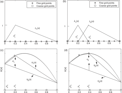
The general idea of the method consists of a step by step approach to the function k_I(x) defined by (13), starting from the first coarse grid point , as follows: (13) where The functions L₁(x) and k₁(x) are plotted in Figure 1(a) and (c), respectively. Next iterations k_m(x) (Figure 1(d)) are defined to be (14) where This iteration process (from m = 1 to m = N_c) is defined to be the exterior iteration process. At each step of this iteration process the unknown parameter κ_m, , needs to be defined. This parameter means the difference between the values of the mth iteration k_m(x) and the initial iteration k₀(x) at the coarse grid point : (Figure 1(c) and (d)), due to the ‘coarse’ Lagrange type piecewise-linear function L_m(x) in expansion (14).

Let us now assume that the functions k_m(x) and k_m−1(x), , are two successive iterations defined by (14), and k₀(x) = k(0)(1 − x) + k(1)x is the initial iteration. Then Δk_m(x) = k_m(x) − k_m−1(x). Substituting these in the integral identity (6) instead of k₁(x) and k₂(x), respectively, we get the following nonlinear integro-differential equation with respect to the unknown function k_m(x): (15) Here, and the final time is taken to be the grid point of the uniform coarse time grid which has the same number of points with the coarse space grid . According to Lemma 2.1, the function ϕ(x, t; k_m) on the left-hand side of (15) is the solution of the adjoint problem (16) The arbitrary control function p(t) is chosen here to be (17) Now we require that the function k_m(x) (i.e. the mth iteration) is the solution of the ICP1, which means that the flux −k_m(0)u_x(0, t; k_m) is assumed to be the measured output data f₀(t), i.e. f₀(t) = −k_m(0) u_x(0, t; k_m) . This requirement means that Δf₀(t) = f₀(t) − [−k_m−1(0)u_x(0, t; k_m−1)] on the right-hand side of the integral equation (15).

Using the approximation formula (14) we can express Δk_m(x) via the parameters κ_m and κ_m−1 as follows: Substituting this in (15) we obtain the following nonlinear algebraic equation with respect to the unknown parameter κ_m: (18) The nonlinear functionals ℳ_m = ℳ_m(κ_m), 𝒩_m = 𝒩_m(κ_m) in (18), and the right-hand side d_m are defined by the following integrals: (19) where u(x, t; k_m−1) is the solution of the direct problem (1) corresponding to the known (already found) coefficient k_m−1(x) in the domain , and ϕ(x, t; k_m) is the solution of the adjoint problem (16) corresponding to the coefficient k_m−1(x).

The same nonlinear algebraic equation (18) will be used for the ICP2 and ICP3 with the differences that in (18) the function u(x, t; k_m−1) will be the solution of the direct problem (3) or (5), and the function ϕ(x, t; k_m) will be the solution of the adjoint problem (20) or (21) respectively.

Thus at each mth step (m = 1, 2, … , N_c) of the coarse grid iteration process, one needs to solve the nonlinear equation (18) in the domain . This step requires solving the corresponding forward problem ((1), (3) or (5)) in with already found coefficient k_m−1(x), as well as a series of adjoint problems ((16), (20) or (21)), as formulas (19) show.

For the numerical solution of the forward and backward parabolic problems the following uniform fine space and time grids, with the grid points , and grid steps , , respectively, are introducesd. These grids consist of the following uniform subgrids Due to the dependence of the adjoint problem solution ϕ(x, t; k_m) on the unknown coefficient k_m(x), the second iteration process needs to be constructed for the numerical solution of adjoint problem (16), (20) or (21), at each mth step of the coarse grid iteration process. With this fine grid iteration process, all iteration process of reconstructing the unknown function k_I(x) is defined to be the coarse-fine grid iteration process.

Note also that the presented method is not a multigrid method, which is usually based on the utilization of several grids of increasing fineness. The main principle of multigrid methods consists of obtaining the solution of a problem posed on the finest grid by successive solutions performed on coarser grids 8. These methods use operators for interpolation (transition from coarse to fine grids), sampling (transition from fine grid to coarse) and smoothing. The corrections effected on the coarse grids are calculated by direct or iterative solvers. The numerical method proposed here uses just two grids: the coarse grid for parameterizing the unknown coefficient, and the fine grid for the numerical solution of the forward and adjoint problems.

3. The coarse-fine grid iteration algorithm (CFGIA) and numerical test examples

Let us apply the following linearization scheme to the nonlinear integro-differential equation (18) with respect to the unknown parameter κ_m, : (22) Note that for m = 1, Equation (18) and its linearization have more simple forms: (23)

With the above simple iteration algorithm the coarse-fine grid iteration process can be summarized as follows.

Algorithm (CFGIA)

	(i1) Generate the initial iteration k0(x) = k(0)(1 − x) + k(1)x for coarse grid iteration process (m = 0);
	(i2) Use (24) to find the parameter κ1: apply here the fine grid iteration process for calculating (m = 1);
	(i3) Repeat the coarse grid iteration process from m = 2 to m = Nc for solving the linearized algebraic equation (23);
	(i4) At each mth step () of (i3) use the fine grid iteration process for calculating and in (23);
	(i5) Use formula (13) and reconstruct the function kI(x) for the found parameters κm, .

The following quantity is defined for the Algorithm (CFGIA): (24)

The above algorithm is tested on all three types of inverse problem to find out:

a.	the optimal number Nc of basis functions in the sense of optimal compromise between the accuracy and stability of the inverse problem solution;
b.	the influence of input sources on the reconstruction of the unknown coefficient;
c.	similarities and differences of solutions of the ICP1, ICP2 and ICP3 for the same input data.

In all the numerical test examples the output data f₀(t) and ν₀(t) for the above formulated inverse problems are generated from the numerical solutions of corresponding direct problems, giving the coefficient k(x) and the appropriate input data ν₀(t) or f₀(t). For this the finite-difference schemes proposed in 7 are used. Specifically, the finite-difference analogue of the direct problem (1) is the following discrete problem: (25) For a given input data k(x) and ν₀(t), the discrete values of the output data f₀(t) are generated from the numerical solution of the discrete problem (25) by the following difference scheme: (26) Similar discrete problems are used for the ICP2 and ICP3 7, formulas (37) and (38)].

Example 1

Let us analyse first the sensitivity of the considered inverse problems with respect to the coarse grid size N_c. For this aim, the Algorithm (CFGA) is performed on two different coarse meshes with parameters N_c = 19 and N_c = 28 (the corresponding fine mesh parameters are h = 0.005, τ = 0.0025 and h = 0.0034, τ = 0.0017). The functions k(x) = 9x³ − 9x² + x + 1 and lbd(t) = −exp(−50(t − 0.25)²) are used as given input data in the direct problems (1), (3) and (5) (lbd(t) = ν₀(t) in (1), and lbd(t) = f₀(t) in (3) and (5)). Solving these problems the appropriate synthetic (measured) output data and are generated for the ICP1, ICP2 and ICP3.

Figure 2(a) and (b), corresponding to N_c = 19 and N_c = 28, illustrate reconstruction of the coefficient k(x) from the numerical solutions of the ICP1, ICP2 and ICP3. The relative errors δ_k ≔ ‖(k − k_I)/k‖₀ in L₂-norm, corresponding to each inverse problem, are given in Table 1. These results show, first of all, that the reconstructions obtained on both coarse grids are almost the same. Moreover, numerical experiments show that the accuracy of reconstruction of the coefficient k(x) for all coarse grids with parameters N_c = 11 ÷ 19 are also almost the same. Hence these parameters are acceptable and can be used in subsequent computational experiments. Further, in the considered example relative errors δ_k, corresponding to the ICP1 and ICP2, are very close, while relative errors corresponding to the ICP3 are slightly greater. Different from ICP1, in the case of ICP2 and ICP3, detoriations can be observed at the points close to the right end x = 1. Comments related to this phenomenon will be given below.

Note that in all the numerical examples the number of iterations in (24), corresponding to the stopping parameter , was about 5 ÷ 7.

Figure 2. Reconstruction of the coefficient k(x) = 9x³ − 9x² + x + 1 from numerical solutions of the ICP1, ICP2 and ICP3 on the coarse grids with grid parameters N_c = 19 (a) and N_c = 28 (b).

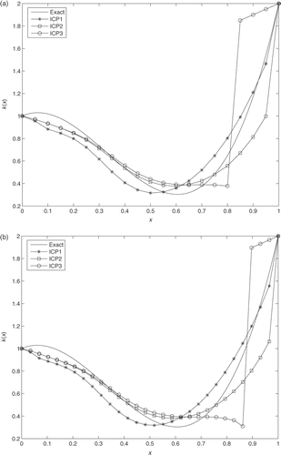
Table 1. Relative errors δ_k in L₂-norm.

Nc	ICP1	ICP2	ICP3
19	0.19	0.16	0.33
28	0.20	0.16	0.26

Example 2

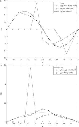
To analyse the influence of the character of the input data ν₀(t) on the reconstruction of the unknown coefficient function k(x), two types of Dirichlet input data are taken in the ICP1: the smooth function ν₀(t) = exp(−100(t − 0.5)²) and the Dirac function ν₀(t) = 100δ(t − t₀), with t₀ = 0.5 and t₀ = 0.25. In the first series of numerical examples the synthetic output data , defined by (27), are generated for the coefficient k(x) = 1 + 0.5 sin(2πx). Numerical results corresponding to the smooth input data ν₀(t) = exp(−100(t − 0.5)²), and to the Dirac input data ν₀(t) = 100δ(t − 0.5) and ν₀(t) = 100δ(t − 0.25) are illustrated in the left of Figure 3. For the smooth input data the reconstruction of the unknown coefficient k(x) is high enough and the relative error is δ_k = 2.8 × 10⁻². However, detoriations are observed in the case of both Dirac input data, as shown in Figure 3(a). Similar results are obtained in the case of the coefficient k(x) = 1 + 0.25 sin(πx) (Figure 3(b)). Hence an input data ν₀(t) of δ-function type is not acceptable for the Algorithm (CFGA), although any approximation of this data by the functions , α, β > 0 is acceptable.

Figure 3. Exact and numerical solutions of the ICP1 for various left boundary functions ν₀(t). (a) k(x) = 1+0.5 sin(2πx) and (b) k(x) = 1 + 0.25 sin(πx).

Example 3

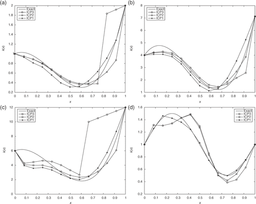
To make a comparison between the ICP1, ICP2 and ICP3, the Algorithm (CFGA) with coarse grid parameter N_c = 11 is applied to these problems. The noise free synthetic output data are generated from the following coefficient k(x) and the left boundary data (lbd(t)) in appropriate direct problems:

The depth of concavity of each function k(x) is taken to be different. Numerical results plotted in Figure 4 show that the best reconstruction is obtained from the numerical solution of ICP1. The quality of these reconstructions also depends on deepness of the concavity: less concavity leads to better reconstruction. In the case of ICP2 and ICP3, deviations occur at the points close to the right end x = 1. The reason apparently is that the input data in the ICP2 and ICP3 is of Neumann type. As a result, the boundary condition(s) in the corresponding adjoint problems are also of Neumann type. Since at each mth step of the coarse grid iteration process the fine grid iteration process requires solving these adjoint problems, due to these Neumann conditions accumulation of computational errors occurs. This leads to the above mentioned deviations.

Figure 4. Exact and numerical solution of the ICP1-ICP3 for various coefficients k(x). (a) Reconstruction of the coefficient function , (b) reconstruction of the coefficient function , (c) reconstruction of the coefficient function and (d) reconstruction of the coefficient function .

Example 4

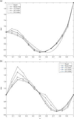
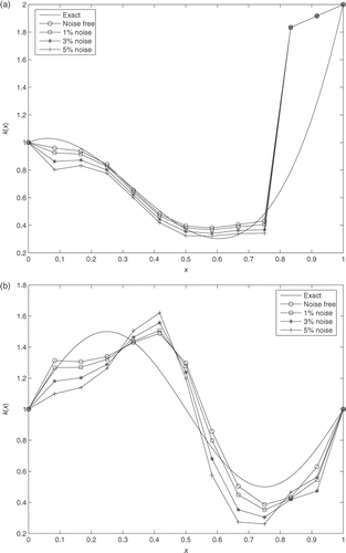
To analyse the sensitivity of the Algorithm (CFGA) the ICP1 and ICP3 are tested with the noisy data containing 1%, 3% and 5% random noise levels. The noise free data for these inverse problems are generated from the given coefficients k⁽¹⁾(x) = 9x³ − 9x² + x + 1 and k⁽⁴⁾(x) = 1 + 0.5 sin(2πx), and the input data lbc⁽¹⁾(t) = −exp(−100(t − 0.25)²) and lbc⁽⁴⁾(t) = −exp(−100(t − 0.5)²). These input data are taken as the left boundary data ν₀(t) and f₀(t) in the direct problems corresponding to the ICP1 and ICP3, respectively. Figures 5 and 6 illustrate the numerical solutions of these inverse problems corresponding to noise free and noisy data. The relative errors are reported in Table 2. These results show that both inverse problems have the same sensitivity with respect to noise.

Figure 5. Noise analysis for ICP1. (a) and (b) .

Figure 6. Noise analysis for ICP3. (a) and (b) .

Table 2. L₂-norm relative errors δ_k for the ICP1 and ICP3.

	Noise free data	Noisy data	Noisy data	Noisy data
ICP1
k^(1)(x) = 9x^3 − 9x^2 + x + 1	0.18	0.17	0.15	0.14
k^(4)(x) = 1 + 0.5 sin(2πx)	0.023	0.042	0.12	0.20
ICP3
k^(1)(x) = 9x^3 − 9x^2 + x + 1	0.42	0.42	0.43	0.43
k^(4)(x) = 1 + 0.5 sin(2πx)	0.16	0.19	0.24	0.27

5. Conclusions

The aim of this article was to demonstrate an implementation of the coarse-fine grid algorithm to inverse coefficient problems with boundary measured data. Although all types of inverse coefficient problems are severely ill-posed, the presented computational results show that this ill-posedness slightly depends on where the Neumann and Dirichlet conditions are given: in the direct problem or as measured output data. Specifically, use of Dirichlet conditions in the direct problem as input data, and Neumann conditions as output data (the ICP1) lead to better reconstructions.

Computational experiments show that values N_c = 11 ÷ 28 of the coarse grid parameter N_c guarantee an optimal compromise between the accuracy and stability of the numerical solution of inverse problems. Further increase in this parameter (N_c > 30) leads to detoriations, even in the case of noisy free output data. The reason for this phenomenon is that Equation (18) is a nonlinear one with respect to the unknown parameter κ_m and the functionals ℳ_m and 𝒩_m, defined by (19), use the parameter κ_m−1 found from the previous (m − 1)th iteration. Each of these parameters contain computational errors. By increasing the number of iterations m, these errors accumulate, and the second noise factor - computational noise factor – arises.

Numerical examples presented here for various coefficients and input data show the feasibility of implementation of the integral identities, and an effectiveness of the Algorithm (CFGA) based on these identities. However, the input data of δ-function type (pointwise input source) is not acceptable for the Algorithm (CFGA), as the presented results show. However, any approximation of this data by the functions , α, β > 0 is acceptable. Numerical solution of the above inverse coefficient problems with the input data of δ-function type will be given in Part III.

Acknowledgements

This research has been supported by the Scientific and Technological Research Council of Turkey (TUBITAK) through the project no. 108T332. The work of Alemdar Hasanov has also been supported by the International Research Program of L.N. Gumilev Eurasian National University, Astana, Kazakhstan. The authors thank the referees whose comments and suggestions substantially improved the revision of this article.

References

- DuChateau, P, 1995. Monotonicity and invertibility of coefficient-to-data mappings for parabolic inverse problems, SIAM J. Math. Anal. 26 (1995), pp. 1473–1487.
- DuChateau, P, 1996. "Introduction to inverse problems in partial differential equations for engineers, physicists and mathematicians". In: Gottlieb, J, and DuChateau, P, eds. Parameter Identification and Inverse Problems in Hydrology, Geology and Ecology. Dordrecht: Kluwer Academic Publishers; 1996. pp. 3–38.
- DuChateau, P, 1997. An inverse problem for the hydraulic properties of porous media, SIAM J. Math. Anal. 28 (1997), pp. 611–632.
- DuChateau, P, Thelwell, R, and Butters, G, 2004. Analysis of an adjoint problem approach to the identification of an unknown diffusion coefficient, Inverse Problems 20 (2004), pp. 601–625.
- Hasanov, A, DuChateau, P, and Pektas, B, 2006. An adjoint problem approach and coarse-fine mesh method for identification of the diffusion coefficient in a linear parabolic equation, J. Inverse Ill-Posed Problems 14 (5) (2006), pp. 435–463.
- Hasanov, A, Demir, A, and Erdem, A, 2007. Monotonicity of input-output mappings in inverse coefficient and source problems for parabolic equations, J. Math. Anal. Appl. 335 (2007), pp. 1434–1451.
- Hasanov, A, Pektas, B, and Erdem, A, 2011. Comparative analysis of inverse coefficient problems for parabolic equations, Part I: Adjoint problem approach, Inverse Problems Sci. Eng. 19 (2011), pp. 599–615.
- Wesseling, P, 1992. An Introduction to Multigrid Methods. New York: Wiley; 1992.