Numerical approximation of the one-dimensional inverse Cauchy–Stefan problem using a method of fundamental solutions

Abstract

We investigate an application of the method of fundamental solutions (MFS) to the one-dimensional parabolic inverse Cauchy–Stefan problem, where boundary data and the initial condition are to be determined from the Cauchy data prescribed on a given moving interface. In [B.T. Johansson, D. Lesnic, and T. Reeve, A method of fundamental solutions for the one-dimensional inverse Stefan Problem, Appl. Math Model. 35 (2011), pp. 4367–4378], the inverse Stefan problem was considered, where only the boundary data is to be reconstructed on the fixed boundary. We extend the MFS proposed in Johansson et al. (2011) and show that the initial condition can also be simultaneously recovered, i.e. the MFS is appropriate for the inverse Cauchy-Stefan problem. Theoretical properties of the method, as well as numerical investigations, are included, showing that accurate results can be efficiently obtained with small computational cost.

Keywords:

• heat conduction
• method of fundamental solutions
• inverse Cauchy–Stefan problem

AMS Subject Classifications:

• 35K05
• 35A35
• 65N35
• 80A22

1. Introduction

The method of fundamental solutions (MFS) is a powerful numerical technique, which is meshfree and, compared to other popular numerical techniques, is easy to use and has small computational cost, for a review see 1. The method can be applied to both direct and inverse problems, and in this article we focus on the inverse Cauchy–Stefan problem. Stefan problems, both direct 2 and inverse 3, model many real world and engineering situations, including the melting of ice, solidification of metals, casting, ablation, etc. The direct Stefan problem usually requires determining both the temperature and free boundary when the initial and boundary conditions are known along with the thermal properties. On the other hand, there are several inverse Stefan problems that can be formulated, and these usually require determining initial and/or boundary conditions, and/or the free boundary, for example, the inverse boundary Stefan problem, the inverse Cauchy–Stefan problem and the inverse Stefan problem. For more details on Stefan problems, see 4–11.

Recently, the authors of this article have obtained numerical results for the inverse Stefan problem using an MFS where boundary data was reconstructed on the fixed boundary knowing the initial conditions and the moving interface, see 12. As was pointed out in 13,14, the knowledge of the initial condition is in theory not needed for the recovery of the boundary data in the inverse Stefan problem. The inverse problem of simultaneously finding the initial data and boundary data is termed the inverse Cauchy–Stefan problem. We extend the MFS of 12 to the inverse Cauchy–Stefan problem, and shall compare the numerical reconstructions in 12 with those obtained here when the initial condition is not specified. Similar MFS investigations, with or without initial value prescribed, have been considered in 15,16 for the inverse boundary Stefan problem, and in 17,18 for the inverse heat conduction problem with s(t) ≡ constant function.

The outline of this article is as follows: in Section 2, we give a mathematical formulation for the inverse Cauchy–Stefan problem. In Section 3, we describe an MFS for solving this problem and state denseness results for this MFS approximation. Three numerical examples are given and investigated in Section 4, displaying the accuracy of the MFS for the inverse Cauchy–Stefan problem, and showing that the initial condition is indeed not needed to obtain accurate and stable results.

2. The inverse Cauchy–Stefan problem

We consider a one-dimensional setting in space and denote the free boundary (sufficiently smooth) by Γ_S given through the equation x = s(t), for 0 < t ≤ T, where T is an arbitrary final positive time. We assume that s(t) > 0 for t ∈ (0, T] and s(0) ≥ 0. The heat conduction domain is D = (0, s(t)) × (0, T ] with closure . We put Γ_U = ({0} × (0, T)) ∪ ((0, s(0)) × {0}) and data on this portion will not be specified.

For the inverse Cauchy–Stefan problem we wish to determine a solution that satisfies the one-dimensional heat equation (1) subject to the given Dirichlet and Neumann boundary conditions on the moving boundary Γ_S (where x = s(t)) according to (2) (3) In Stefan problems, usually h₁(t) = 0 and h₂(t) = −s′(t).

The aim is then to reconstruct the initial value of the solution at t = 0, as well as its value and the normal derivative at the fixed boundary x = 0, i.e. to find u₀(x), f(t) and g(t) with (4) (5) (6) If s(0) = 0 then the initial condition (4) is not involved.

A result about a priori (which assumes a solution exists) and a posteriori estimates, and hence uniqueness, can be found in 19, and is stated in the following theorem.

Theorem 2.1

If is a solution of (1–3) for s ∈ C¹([0, T ]) and h₁, h₂ ∈ C²([0, T ]), then there exists a function θ(x) > 0 for x ∈ (0, s(t)), and a constant C = C(M, μ, δ) > 0 such that (7) for any δ ∈ (0, T ], where M = max{∥u∥, ∥u_x∥}, μ = min_τ∈[0,T] s(τ), and ∥ · ∥ denotes the maximum continuity norm on a compact interval.

For the non-characteristic Cauchy problem (1–3) with analytic s, h₁ and h₂, we can rearrange the Cauchy–Kowalewski series to formally obtain, see 20 and 21, Theorem 2.6.1], the solution (8)

In the case of the Stefan problem with h₁(t) = 0 and h₂(t) = −s′(t), Equation (8) simplifies to (9) For s(0) > 0 the formal solution (8) is also a solution to the inverse Stefan problem (1–4) if the initial data u₀(x) fits the limit, as t tends to zero, of (8). However, formula (8) is not useful numerically since it involves infinite differentiation of functions which are seldom smooth in practice. Therefore, in this article we propose an MFS to simultaneously determine the missing initial data u₀(x) and the boundary data f(t) and g(t) in (4–6). Finally, note that in the particular case when s(t) is a constant function, the non-characteristic Cauchy problem (1–3) has been very recently investigated in 18.

3. The MFS

Over the past few years the MFS has become an increasingly popular numerical technique, used for solving linear partial differential equations (PDEs) when the fundamental solution is available explicitly. Mostly, the MFS has been used to solve elliptic linear PDEs, including Laplace, Helmholtz, convection–diffusion, biharmonic, Lamé, Stokes equations 2,22–24; however, it has only recently been applied to parabolic (linear) PDEs, for example the heat equation, 25–31.

The fundamental solution to the one-dimensional heat equation (1) is given by (10) where H is the Heaviside function. We shall build an approximation to (1–3) using F in (10) as a basis function.

3.1. The MFS and denseness properties

We shall construct a set of source points located external to the domain D. These points will be located on the set Γ_E, which is the union of the boundaries , given by x = y₁(t), with y₁(t) < 0, and , given by x = y₂(t), with y₂(t) > s(t), for t ∈ (−T, T). A restriction we make, such that denseness results hold for the MFS that we shall propose, is that y₂(τ) − s(0) > 0 for all τ < 0. For more on the placement of source points, in the stationary case, see, for example, 32,33.

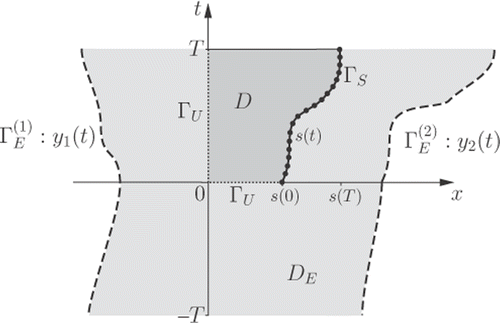
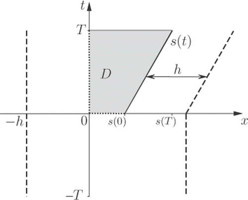
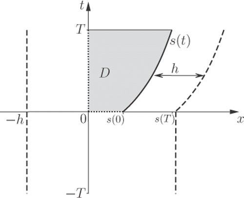
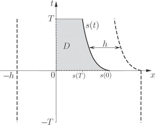
We denote by D_E the domain contained within the boundary Γ_E for t ∈ (−T, T). We shall then place source points on Γ_E and collocation points on the moving boundary Γ_S. For a visual representation of a general domain and possible location of collocation and source points, see Figure 1.

Figure 1. General representation of the domain D and boundary Γ = Γ_U ∪ Γ_S, with unspecified initial and boundary conditions (·····) on Γ_U, collocation points () on Γ_S and source points (- - -) placed on external to the domain D.

Let {(y_j(τ_m), τ_m)}_{m=1, 2, …} for j = 1, 2 be a denumerable, everywhere dense set of source points equally distributed on the external boundary Γ_E. To be able to define an MFS approximation valid also at t = 0, we assume that τ_m ≠ 0 for m = 1, 2, …. The MFS approximation we propose, which satisfies Equations (1–3), is a linear combination of fundamental solutions (10), given by (11) The unknown constants are set equal to zero, except for a finite number of values; note that u_∞(x, t) = 0 for because of the Heaviside function in (10). Linear independence and denseness results were proved in 26,34 to justify the MFS representation (11) and are stated in the following theorem.

Theorem 3.1

Elements of the form (11) constitute a linear independent and dense set in the L²-sense on the boundaries Γ_U and Γ_S.

Note that this result has been generalized to two-dimensional solution domains in 35.

3.2. Specification of collocation and source points

To implement the MFS for the inverse Cauchy–Stefan problem we first truncate (11) by taking a finite number of terms, namely (12)

We then place M + 1 (M even) collocation points on the lateral surface Γ_S (the moving interface) given by There are then M + 1 collocation points on Γ_S, where, according to (2)–(3), both the Dirichlet and Neumann conditions will be applied. Therefore, we place 2M + 2 source points external to the domain and equally distributed on the boundary Γ_E (see Figure 1). To specify these source points let be given by We note that the points τ_m have been placed between every other time point for t > 0, and moreover τ_m ≠ 0. The remaining M/2 + 1 points are equally distributed on the interval (−T, 0). We point out that the distribution of points on the interval (−T, 0) has little influence on the numerical approximation. The source points on Γ_E are then specified by defining y₁(τ_m) and y₂(τ_m) as (13) where h > 0 is a parameter to be prescribed. The location and number of collocation and source points are different to those in 12 to adjust to the fact that the initial condition is not specified in the inverse Cauchy–Stefan problem.

We impose the Dirichlet and Neumann boundary conditions (2)–(3) to determine the constant coefficients in (12), and obtain the following system of linear algebraic equations (14)

We can represent the system of equations above by (15) where the vector c denotes the unknown constants , g represents the boundary values at the corresponding collocation points and A is the matrix denoting values of the fundamental solution and its x-derivative. Here, A is a square matrix of size (2M + 2) × (2M + 2).

A usual feature of the MFS is the ill-conditioning of the matrices generated, see 36,37, therefore regularization is required when solving (15). There are some ways to handle ill-conditioned matrices, in particular the truncated singular value decomposition, or, the method we choose, Tikhonov's regularization, which solves the modified system of equations (16) instead of (15), where the superscript tr denotes the transpose of a matrix and I is the identity matrix. For exact input data (14), the regularization parameter λ is usually as small as possible or even equal to zero for some configurations; however, care must be taken when noise is added into the boundary data (14). We note that there are methods for choosing the regularization parameter λ, and in this article we use the heuristic L-curve criterion described in 38.

4. Numerical results

4.1. Example 1

We shall first investigate Example 1 from 12, when the initial data is not given. We recall from 12,39 that the free boundary is given by the linear function (17) We place source points according to (13) on the external boundaries (−h, τ), τ ∈ (−1, 1), (s(τ) + h, τ), τ ∈ [0, 1) and (s(0) + h, τ), τ ∈ (−1, 0); for an illustration see Figure 2. We use the solution to the heat equation in D, given by (18) to generate the input data. Therefore, in this example, we have the following boundary conditions on the moving interface: (19) (20)

Figure 2. Particularization of Figure 1 for s(t) given by Equation (17) in Example 1.

Random additive noise is added to the Neumann data (20) as follows: (21) where N(0, σ²) represents the normal distribution with mean zero and standard deviation (22) where δ is the relative (percentage) noise level.

We wish to determine the initial condition at t = 0, as well as the Dirichlet and Neumann conditions along x = 0, given, respectively, by (23) (24)

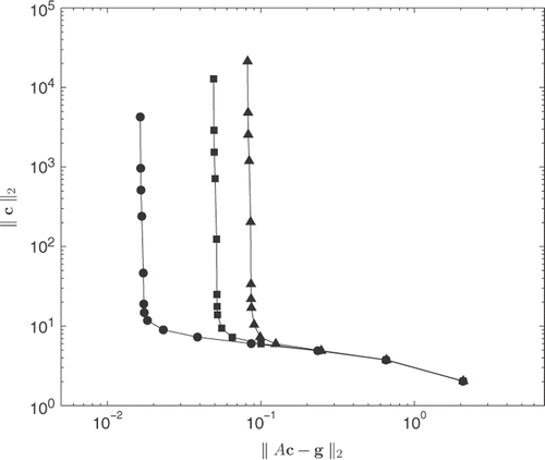
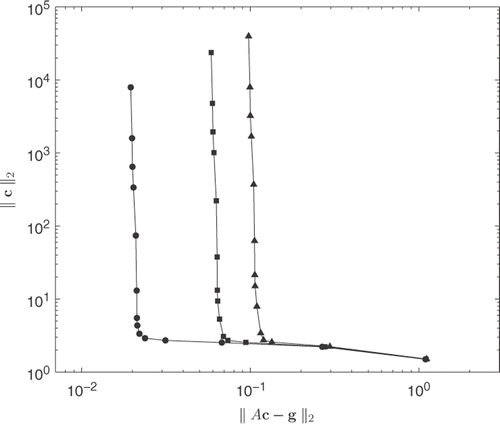
Figure 3 shows plots of the L-curve for different noise levels, and by considering the vertex of the ‘L’, as suggested by Hansen 38, we choose λ = 10⁻⁶ for δ = 1%, and λ = 10⁻⁵ for δ = 3% and 5%.

Figure 3. L-curve plots for δ = 1% (—–), δ = 3% () and δ = 5% () when M = 30 in (12), for Example 1.

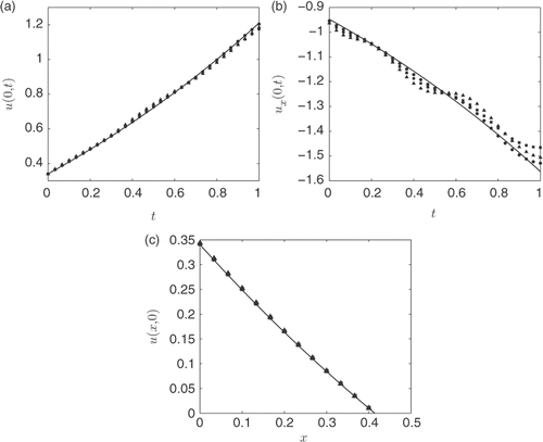
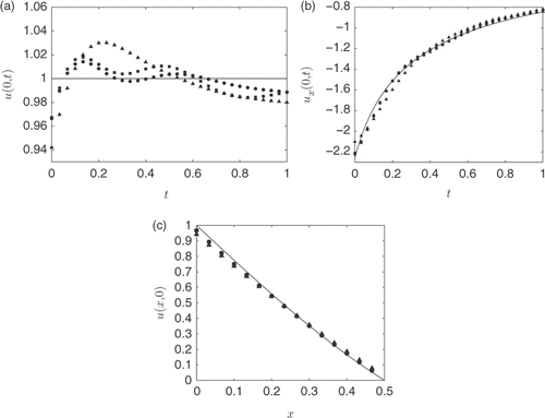
Figure 4(a)–(c) shows plots of the MFS approximations for the reconstructed data u(0, t), u_x(0, t) and u(x, 0), respectively, for noise levels δ ∈ {1, 3, 5}%. First, from Figure 4(c) it can be seen that the numerical MFS results for the initial data are in good agreement with the exact solution (23) and they are relatively insensitive to noise. On the other hand, and rather surprising, but in agreement with the theoretical results of 13, Figure 4(a) and (b) suggests that we have even better results considering the inverse Cauchy–Stefan problem compared to the inverse Stefan problem in 12. There may be a few reasons for this, in particular, a different value of h and other values of the regularization parameter have been chosen, and different sets of random noise have been generated for this example compared to 12. Also, more source points have been placed in time, i.e. M = 30 in this example instead of M = 16 in 12. We note that it is difficult to do a direct comparison with 12, because of the removal of the initial condition and, hence, a change in the number of collocation points, i.e. if M = 16 then the size of the matrix A in 12 is 64 × 64, whilst in this article it is 34 × 34. However, at the end of this example we do compare results when using the similar parameters used in Example 1 of 12.

Figure 4. The exact solutions (—–) and MFS approximations for: (a) u(0, t), (b) u_x(0, t) and (c) u(x, 0). All MFS approximations have been generated for noise levels δ = 1% (•) with λ = 10⁻⁶, δ = 3% (▪) with λ = 10⁻⁵ and δ = 5% (▴) with λ = 10⁻⁵, and obtained with h = 2, and M = 30, for Example 1.

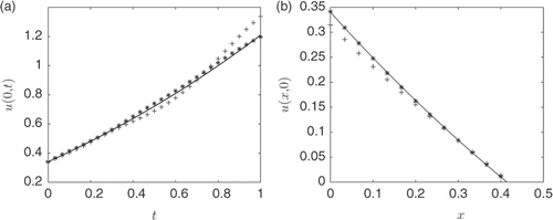
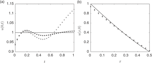
Figure 5(a) and (b) shows plots of the best and least accurate approximations after 10 trials for the MFS approximation of u(0, t) and u(x, 0), respectively. We see similar results as in 12, with errors increasing as t increases. This is to be expected since if we invert the Cauchy data (2) and (3) at x = s(t) collected over the interval [0, T ], we cannot determine accurately the boundary temperature (5) and heat flux (6) at x = 0 for t = T, see 40.

Figure 5. Plots of the exact solution (—–) and the best (*) and least (+) accurate MFS approximations from 10 different sets of noisy data with noise level δ = 5% for (a) u(0, t) and (b) u(x, 0). Both plots are obtained with h = 2, M = 30 and λ = 10⁻⁵, for Example 1.

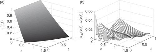
Figure 6(a) shows a plot of the exact solution, and Figure 6(b) shows a plot of the absolute error for the noise level δ = 5%. Even though the numerical solution is slightly oscillatory, the maximum error is relatively low, and of the same order, compared to the noise level.

Figure 6. (a) The exact solution u(x, t) for all (x, t) ∈ D and (b) the absolute error for all (x, t) ∈ D for noise level δ = 5%, obtained with h = 2, λ = 10⁻⁵, M = 30, for Example 1.

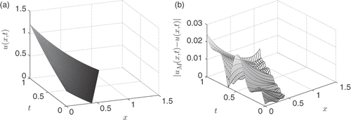
The final two figures for this example are used for comparison with the results obtained in Example 1 of 12 (where the initial data (23) was given). Figure 7(a) and (b) differs only by the number of source and collocation points that have been placed in time (note that the matrix A is still square). Figure 7(a) suggests that a higher value of M in (12) is needed for determining accurately the initial condition, whereas Figure 7(b) gives a very similar result to Figure 9(b) in 12, where the same set of random noise has been applied.

Figure 7. Plots of the absolute error for all (x, t) ∈ D for noise level δ = 5% obtained with h = 2.5, λ = 10⁻⁶ and (a) M = 30 and (b) M = 16, for Example 1.

Figure 8. Particularization of Figure 1 for s(t) given by Equation (25) in Example 2.

Figure 9. L-curve plots for δ = 1% (), δ = 3% () and δ = 5% () when M = 30, for Example 2.

Note that the variables used in this example are not optimized. Thus, another value for h, changes in the number of points M placed in time and different choices for the regularization parameter λ may produce even better results.

4.2. Example 2

The following example was investigated in 26, but with the direct Stefan problem being the focus of that paper. The free boundary in this example is given by the nonlinear function (25) where t₀ = 0.162558 and a = 0.620063. We shall place source points on the external boundaries (−h, τ), τ ∈ (−1, 1), (s(τ) + h, τ), τ ∈ [0, 1) and (s(0) + h, τ), τ ∈ (−1, 0), for an illustration, see Figure 8. We take the solution to the heat equation (1) given by (26) where (27) is the error function. From this we generate the following boundary conditions (2)–(3) on the free boundary: (28) (29)

Noise is then added to the Neumann data (29) similar to (21)–(22).

We wish to determine the output data (4–6) given by (30) (31)

Figure 9 shows plots of the L-curve for different noise levels; by studying the corner of the ‘L’ we choose the regularization parameters λ = 10⁻⁶ for δ = 1%, and λ = 10⁻⁵ for δ = 3% and 5%.

In Figure 10(a)–(c), the MFS approximations for the missing data u(0, t), u_x(0, t) and u(x, 0), respectively, are plotted for noise levels δ ∈ {1, 3, 5}%. We obtain similar stable results as in the previous example. Also the initial condition, which is not supplied, is approximated with good accuracy.

Figure 10. The exact solutions (—–) and MFS approximations for: (a) u(0, t), (b) u_x(0, t) and (c) u(x, 0). All MFS approximations have been generated for noise levels δ = 1% (•) with λ = 10⁻⁶, δ = 3% (▪) with λ = 10⁻⁵ and δ = 5% (▴) with λ = 10⁻⁵, and obtained with h = 2, and M = 30, for Example 2.

Figure 11(a) and (b) shows the best and least accurate approximations after 10 trials for the MFS approximation of u(0, t) and u(x, 0), respectively, however, for one of the sets of random noise the maximum error is relatively large; this may be because the random data contains large values or a better choice of regularization parameter may be required with another plot of the L-curve for that data.

Figure 11. Plots of the exact solution (—–) and the best (*) and least (+) accurate MFS approximations from 10 different sets of noisy data with noise level δ = 5% for (a) u(0, t) and (b) u(x, 0). Both plots are obtained with h = 2, M = 30 and λ = 10⁻⁴, for Example 2.

Finally, Figure 12(a) shows a plot of the exact solution, and we note that the solution has a relatively steep gradient which may affect the accuracy of the approximation at the initial and final time points. Figure 12(b) is a plot of the absolute error for the noise level δ = 5%, and the error is greatest at t = 0, where the solution has its largest gradient. The maximum error obtained, however, is again of the same order as the noise level. Example 2 displays similar features to those of Example 1 and it appears again that not supplying the initial condition has not impaired the results in any significant way.

Figure 12. (a) The exact solution u(x, t) for all and (b) the absolute error for all (x, t) ∈ D for noise level δ = 5%, obtained with h = 2, λ = 10⁻⁵, M = 30, for Example 2.

4.3. Example 3

In this example the MFS is applied to a more difficult problem where we have a singularity in the solution at the initial point (s(0), 0) of the closure of the moving boundary Γ_S. The problem we consider is a modification of Neumann's analytic solution; the unmodified Neumann's analytic solution was, for example, considered in 41. The nonlinear function representing the free boundary is now given by (32) where b = 1/4. We place source points on the external boundaries (−h, τ), τ ∈ (−1, 1), (s(τ) + h, τ), τ ∈ [0, 1) and (s(0) + h, τ), τ ∈ (−1, 0); for an illustration see Figure 13. We use the exact solution given by (33) where erfc(ξ) = 1 − erf(ξ) is the complementary error function. The solution u in (33) has a singularity located at (s(0), 0) = (1, 0). From (33) we generate the following boundary conditions (2)–(3) on the free boundary: (34) (35)

Figure 13. Particularization of Figure 1 for s(t) given by Equation (32) in Example 3.

From (35) it can be seen that the heat flux at x = s(t) blows up to infinity as t tends to zero. We wish to determine the output data (4–6) given by (36) (37)

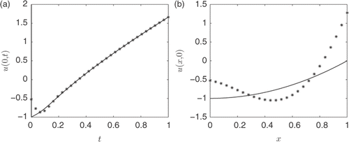
Figure 14(a) and (b) shows plots of the MFS approximation of u(0, t) and u(x, 0), respectively, when noise has not been applied to the boundary data. In Figure 14(a) we can see that the error is larger at small t than elsewhere; this is due to the singularity at (x, t) = (1, 0). Figure 14(b) confirms this, with results being unstable and oscillatory; different choices of λ, M and h did not improve the accuracy significantly.

Figure 14. (a) The exact solution u(0, t) (—–) and the MFS approximation, and (b) the exact solution u(x, 0) (—–) and the MFS approximation. Both plots are obtained with λ = 10⁻⁸, h = 2 and M = 30, for Example 3.

To obtain better results we remove the singularity, as was suggested for different examples with singularities in 28,42. We define (38) which satisfies the heat equation (1), and instead apply the MFS to u* = u − u_sing. The function u* is now regular and satisfies the heat equation (1), and the following modified Dirichlet and Neumann boundary conditions: (39)

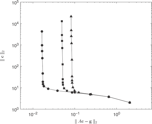
Figure 15 shows plots of the L-curve for different noise levels, and by considering the corner of the ‘L’, we choose the regularization parameters λ = 10⁻⁶ for δ = 1%, λ = 10⁻⁵ for δ = 3%, and 5%.

Figure 15. L-curve plots with the singularity removed for δ = 1% (), δ = 3% () and δ = 5% () when M = 30, for Example 3.

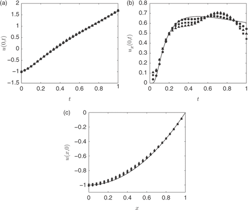
In Figure 16(a)–(c) the MFS approximations for the reconstructions of the data u(0, t), u(0, t) and u(x, 0), respectively, are plotted for noise levels δ ∈ {1, 3, 5}%, with the respective regularization parameters described above. By comparing Figure 14(a) and (b) with Figure 16(a) and (c), respectively, it can be seen that the removal of the singularity (38) has produced significantly more accurate results.

Figure 16. The exact solutions (—–) and MFS approximations with singularity removed for: (a) u(0, t), (b) u_x(0, t) and (c) u(x, 0). All MFS approximations have been generated for noise levels δ = 1% (•) with λ = 10⁻⁶, δ = 3% (▪) with λ = 10⁻⁵ and δ = 5% (▴) with λ = 10⁻⁵, and obtained with h = 2, and M = 30, for Example 3.

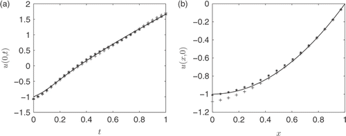
Figure 17(a) and (b) shows the best and least accurate approximations after 10 trials for the MFS approximation of u(0, t) and u(x, 0), respectively, and results are very accurate for all the sets of random data applied to the Neumann boundary data (35).

Figure 17. Plots of the exact solution (—–) and the best (*) and least (+) accurate MFS approximations from 10 different sets of noisy data with noise level δ = 5% for (a) u(0, t) and (b) u(x, 0). Both plots are obtained with the singularity removed, h = 2, M = 30 and λ = 10⁻⁴, for Example 3.

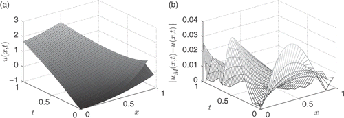
Lastly, Figure 18(a) shows a plot of the exact solution, and Figure 18(b) shows a plot of the absolute error for the noise level δ = 5%. Again, as in the previous examples, we obtain accurate results at the output comparable with the level of noise in the input data.

Figure 18. (a) The exact solution u(x, t) for all and (b) the absolute error for all (x, t) ∈ D for noise level δ = 5%, obtained with the singularity removed, h = 2, λ = 10⁻⁵, M = 30, for Example 3.

5. Conclusion

In this article, an MFS was proposed and investigated for the one-dimensional inverse Cauchy–Stefan problem, where simultaneously initial and boundary data are reconstructed. Three numerical examples were presented showing that the MFS given in 12 to find boundary data can be adjusted to the inverse Cauchy–Stefan problem with some changes to the implementation. In fact, the first example considered is also studied in 12, and the results obtained here demonstrates that knowledge of the initial data is not crucial to get an accurate reconstruction. The third and final example was a more challenging problem since the solution has a singularity located on the boundary of the solution domain. To obtain an accurate MFS approximation it was then necessary to first remove this singularity as was suggested in 28,42.

Acknowledgements

The second author would like to thank the UK Royal Society for the financial support for attending and presenting partial results of this research at the 5th International Conference: Inverse Modeling and Simulation, 24–29 May, 2010, Antalya, Turkey. The third author would like to acknowledge the doctoral training grant received from the EPSRC.

References

- Fairweather, G, and Karageorghis, A, 1998. The method of fundamental solutions for elliptic boundary value problems, Adv. Comput. Math. 9 (1998), pp. 69–95.
- Rubinsteĭn, LI, 1971. The Stefan Problem. Providence, RI: American Mathematical Society; 1971.
- Goldman, NL, 1997. Inverse Stefan Problems. Dordrecht: Kluwer Academic Publishers; 1997.
- Cannon, JR, and Primicerio, M, 1971. Remarks on the one-phase Stefan problem for the heat equation with the flux prescribed on the fixed boundary, J. Math. Anal. Appl. 35 (1971), pp. 361–373.
- Cannon, JR, and van der Hoek, J, 1982. The one phase Stefan problem subject to the specification of energy, J. Math. Anal. Appl. 86 (1982), pp. 281–291.
- Colton, D, and Reemtsen, R, 1984. The numerical solution of the inverse Stefan problem in two space variables, SIAM J. Appl. Math. 44 (1984), pp. 996–1013.
- El Badia, A, and Moutazaim, F, 1999. A one-phase inverse Stefan problem, Inverse Probl. 15 (1999), pp. 1507–1522.
- Jochum, P, 1980. The numerical solution of the inverse Stefan problem, Numer. Math. 34 (1980), pp. 411–429.
- Reemtsen, R, and Kirsch, A, 1984. A method for the numerical solution of the one-dimensional inverse Stefan problem, Numer. Math. 45 (1984), pp. 253–273.
- Slota, D, 2008. Solving the inverse Stefan design problem using genetic algorithms, Inverse Probl. Sci. Eng. 16 (2008), pp. 829–846.
- Slota, D, 2008. Using genetic algorithms for the determination of a heat transfer coefficient in three-phase inverse Stefan problem, Int. Commun. Heat Mass Transfer 35 (2008), pp. 149–156.
- Johansson, BT, Lesnic, D, and Reeve, T, 2011. A method of fundamental solutions for the one-dimensional inverse Stefan problem, Appl. Math. Model. 35 (2011), pp. 4367–4378.
- Cannon, JR, and Hill, CD, 1967. Existence, uniqueness, stability, and monotone dependence in a Stefan problem for the heat equation, J. Math. Mech. 17 (1967), pp. 1–19.
- Hào, DN, 1998. Methods for Inverse Heat Conduction Problems. Frankfurt am Main: Peter Lang; 1998.
- Hon, YC, and Li, M, 2008. A computational method for inverse free boundary determination problem, Int. J. Numer. Methods Eng. 73 (2008), pp. 1291–1309.
- Wei, T, and Yamamoto, M, 2009. Reconstruction of a moving boundary from Cauchy data in one-dimensional heat equation, Inverse Probl. Sci. Eng. 17 (2009), pp. 551–567.
- Hon, YC, and Wei, T, 2004. A fundamental solution method for inverse heat conduction problem, Eng. Anal. Bound. Elem. 28 (2004), pp. 489–495.
- Wang, YB, Cheng, J, Nakagawa, J, and Yamamoto, M, 2010. A numerical method for solving the inverse heat conduction problem without the initial value, Inverse Probl. Sci. Eng. 18 (2010), pp. 655–672.
- Cannon, JR, and Douglas, J, 1967. The Cauchy problem for the heat equation, SIAM J. Numer. Anal. 4 (1967), pp. 317–336.
- Hill, CD, 1967. Parabolic equations in one space variable and the non-characteristic Cauchy problem, Commun. Pure Appl. Maths. 20 (1967), pp. 619–633.
- Cannon, JR, 1984. The One-dimensional Heat Equation. Menlo Park, CA: Addison-Wesley; 1984.
- Balakrishnan, K, and Ramachandran, PA, 2000. The method of fundamental solutions for linear diffusion- reaction equations, Math. Comput. Model. 31 (2000), pp. 221–237.
- Bogomolny, A, 1985. Fundamental solutions method for elliptic boundary value problems, SIAM J. Numer. Anal. 22 (1985), pp. 644–669.
- Golberg, MA, and Chen, CS, 1998. "The method of fundamental solutions for potential, Helmholtz and diffusion problems". In: Golberg, MA, ed. Boundary Integral Methods: Numerical and Mathematical Aspects. Southampton: Computational Mechanics Publications; 1998. pp. 103–669.
- Chantasiriwan, S, 2006. Methods of fundamental solutions for time-dependent heat conduction problems, Int. J. Numer. Methods Eng. 66 (2006), pp. 147–165.
- Chantasiriwan, S, Johansson, BT, and Lesnic, D, 2009. The method of fundamental solutions for free surface Stefan problems, Eng. Anal. Bound. Elem. 33 (2009), pp. 529–538.
- Golberg, MA, Chen, CS, and Muleshkov, AS, , The method of fundamental solutions for time-dependent problems, in Proceedings of 13th International Conference on Boundary Element Technology, C.S. Chen, C.A. Brebbia and D.W. Pepper, eds., WIT Press, Southampton, 1999, pp. 377–386.
- Johansson, BT, and Lesnic, D, 2008. A method of fundamental solutions for transient heat conduction, Eng. Anal. Bound. Elem. 32 (2008), pp. 697–703.
- Johansson, BT, and Lesnic, D, 2009. A method of fundamental solutions for transient heat conduction in layered materials, Eng. Anal. Bound. Elem. 33 (2009), pp. 1362–1367.
- Valtchev, SS, and Roberty, NC, 2008. A time-marching MFS scheme for heat conduction problems, Eng. Anal. Bound. Elem. 32 (2008), pp. 480–493.
- Young, DL, Tsai, CC, Murugesan, K, and Fan, CM, 2004. Time-dependent fundamental solutions for homogeneous diffusion problems, Eng. Anal. Bound. Elem. 28 (2004), pp. 1463–1473.
- Gorzelańczyk, P, and Kołodziej, JA, 2008. Some remarks concerning the shape of the source contour with application of the method of fundamental solutions to elastic torsion of prismatic rods, Eng. Anal. Bound. Elem. 32 (2008), pp. 64–75.
- Alves, CJS, 2009. On the choice of source points in the method of fundamental solutions, Eng. Anal. Bound. Elem. 33 (2009), pp. 1348–1361.
- Kupradze, VD, 1964. A method for the approximate solution of limiting problems in mathematical physics, U.S.S.R. Comput. Math. Math. Phys. 4 (1964), pp. 199–205.
- Johansson, BT, Lesnic, D, and Reeve, T, 2011. A method of fundamental solutions for two-dimensional heat conduction, Int. J. Comput. Math. 88 (2011), pp. 1697–1713.
- Chen, CS, Cho, HA, and Golberg, MA, 2006. Some comments on the ill-conditioning of the method of fundamental solutions, Eng. Anal. Bound. Elem. 30 (2006), pp. 405–410.
- Ramachandran, PA, 2002. Method of fundamental solutions: singular value decomposition analysis, Commun. Numer. Methods Eng. 18 (2002), pp. 789–801.
- Hansen, PC, 1992. Analysis of discrete ill-posed problems by means of the L-curve, SIAM Rev. 34 (1992), pp. 561–580.
- Murio, DA, 1992. Solution of inverse heat conduction problems with phase changes by the mollification method, Comput. Math. Appl. 24 (1992), pp. 45–57.
- Eldén, L, 1983. "The numerical solution of a non-characteristic Cauchy problem for a parabolic equation". In: Deuflhard, P, and Hairer, E, eds. Numerical Treatment of Inverse Problems in Differential Equations and Integral Equations. Basel: Birkhauser; 1983. pp. 246–268.
- Liu, J, and Guerrier, B, 1997. A comparative study of domain embedding methods for regularized solutions of inverse Stefan problems, Int J. Numer. Meth. Eng. 40 (1997), pp. 3579–3600.
- Lesnic, D, Elliott, L, and Ingham, DB, 1995. Treatment of singularities in time-dependent problems using the boundary element method, Eng. Anal. Bound. Elem. 16 (1995), pp. 65–70.