A finite element model for the data completion problem: analysis and assessment

Abstract

We investigate the computational advantages of the Steklov-Poincaré variational formulation, based on the uniqueness Holmgren theorem, for the badly ill-posed data completion problem. We study the discrete solution with a finite element approximation. The uniqueness issue is dealt with and we check that it is related to a discrete Holmgren result which requires a particular assumption on the mesh. Then, the important point is to show how the finite element variational problem may be recast into a least-squares problem. Lavrentiev's method turns out to be a Tikhonov regularization of an ‘underlying’ equation that will never be explicited. When employed in conjunction with the Morozov discrepancy principle to select the regularization parameter, the overall mathematical studies realized specifically for the Tikhonov method extends as well to the Lavrentiev method to conclude to a convergent regularization strategy. Similarly, the conjugate gradient method (CGM) may be considered as applied to a normal equation of that same ‘hidden underlying’ problem. We conduct a brief discussion about this method to explain why it yields a convergent strategy. We close with several numerical simulations for different geometries to assess the Lavrentiev finite element or the PCG finite element solution of the data completion problem.

Keywords:

• finite element solution
• discrete Holmgren principle
• Lavrentiev regularization
• conjugate gradient regularization
• Morozov discrepancy principle

1. Introduction

Growing interest is being paid to the severe ill-posed Cauchy problem, modelling the reconstruction of lacking data on a part of the boundary because of inaccessibility to measures. The recent (and less recent) publications on the subject mark such an interest (see, e.g. 1–16). To tackle it numerically, several approaches have been followed. Some come from formulating the problem as an optimal control model 17, others proceed by iterating alternately between two ad hoc problems, each of them transmitting to the other an appropriate boundary condition on the incomplete boundary 1,18,19, a third category uses the Backus–Gilbert method applied to a moment formulation of the problem 20 and some authors consider the quasi-reversibility method which handles a fourth-order partial differential equation consistent with the initial Laplace equation 21–23. More recently, in 24 and 25, a specific variational framework, relying on the Holmgren uniqueness theorem, has been introduced to handle the Cauchy problem which enables a substantial knowledge of its particularities. The primary objective of this article is to bring out the practical relevance of that variational form when a finite element approximation is intended and numerical computations are to be carried out. Especially appreciable is the fact that the stiffness matrix, obtained from a Galerkin discretization of that variational problem, is square, symmetric and non-negative definite. After a finite element discretization is realized, there comes the issue of solving the discrete problem on computers, and this cannot be securely achieved without a performing regularization strategy. Indeed, data are fatally contaminated by errors and cease to be exact. As a consequence, the existence fails and expecting any crude numerical method to give reasonable results turns out to be absurd without further methodological work. Users need to call for some artifices to be able to safely solve the algebraic system and to produce satisfactory solutions. To realize a trade-off between fitting the Cauchy data and controlling the solution norm, the Lavrentiev method seems naturally fitted because of the symmetry and the non-negative definiteness of the problem. To complete the process and ensure both accuracy and stability, we therefore need an efficient rule in the selection of that parameter. The Morozov discrepancy principle is therefore discussed. Following 26,27, it is not secured that the Lavrentiev method will result in a convergent strategy. Nevertheless, things happen as best as possible since we show that the Lavrentiev regularization coincides in reality with the Tikhonov method for some least squares problem that we call the ‘underlying’ problem.

This article is articulated as follows. In Section 2, we apply the finite element method to the condensed variational formulation of the problem introduced and studied in 24. It is set on the incomplete boundary where unknown data are sought for. We check out the symmetry and the non-negative definiteness of the variational problem. We state the existence of the discrete solution. We explain why that solution almost surely blows up for small size meshes, and resorting to a regularization procedure is hence mandatory. In Section 3, we put the problem under a matrix form. The stiffness matrix enjoys several attractive characteristics, it is square, symmetric and non-negative. We propose a Jacobi preconditioner based on a splitting of that stiffness matrix that turns out to be advantageous in the computational experiences. Then comes the milestone of our study. On account of the symmetry, the non-negativeness so as to the existence result, the matrix equation may be viewed as the normal equation related to another auxiliary problem. Although that problem is not explicit, we are able to prove that a small perturbation on the exact Cauchy data causes a small deviation of the auxiliary data vector.1 As a result, Lavrentiev regularization of the original problem may be seen a Tikhonov method for the ‘underlying’ problem. Section 4 is precisely dedicated to the Lavrentiev method used in conjunction to the Morozov discrepancy principle which results in a convergent strategy. Similarly, in Section 5 we check out why the conjugate gradient method (CGM) employed for the discrete problem associated with the discrepancy principle yields a convergent strategy as well. The numerical exploration in the finite element context of the two regularizations strengthened by the discrepancy principle as a parameter selection rule is undertaken in Section 6. Numerous examples presented there corroborates the efficiency of the variational formulation adopted for our computations in addition to the flexibility and the ease of implementing it.

Some notations. Let x denote the generic point of Ω. The Lebesgue space of square integrable functions L²(Ω) is endowed with the natural inner product ; the associated norm is . The Sobolev space H¹(Ω) involves all the functions that are in L²(Ω) so as their first order derivatives. It is provided with the norm , and the semi-norm is denoted by . Let Υ ⊂ ∂Ω be a connected component of the boundary, the space H^1/2(Υ) is the set of the traces over Υ of all the functions of H¹(Ω) and we adopt the notation H^−1/2(Υ) for the dual space of H^1/2(Υ). We refer to 28 for a detailed study of the fractionary Sobolev spaces.

2. Variational problem and finite elements

Let Ω be a bounded domain in ℝ^d(d = 2, 3) with n being the unit normal to the boundary Γ = ∂Ω oriented outward. Assume that given a partition of Γ into two disconnected parts Γ_C and Γ_I, which means that (Figure 1). This simple partition is made only for convenience. We may have a Dirichlet, Neumann or Robin portion of the boundary. The analysis we conduct in the forthcoming sections may be extended as well.

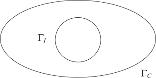
Figure 1. An example of the geometry. Γ_I is unreachable.

Assume a given flux ϕ and a data g. The data completion problem for the elliptic second order operator may be expressed as a Cauchy problem: find u such that (1) (2) (3) a(·) ∈ L^∞(Ω) is bounded away from zero that is a(x) ≥ a_* > 0, ∀x ∈ Ω, with two conditions on Γ_C. The point is to complete the boundary data so as to enable access to the full u by solving a direct problem. Since the lectures by Hadamard in 1922 29, the case of arbitrary domains is successfully considered in a recent work 30 where the severe ill-posedness is established. Moreover, in 24, a variational formulation of the problem is introduced which brings about a deeper theoretical insight on the Cauchy problem. In particular, it is proven there that the set of the non-exact Cauchy data (g, ϕ), for which the existence of solution fails in H¹(Ω), is dense in H^1/2(Γ_C) × H^−1/2(Γ_C). Therefore, it is highly probable that a small pollution will affect any exact couple of data (g, ϕ) and the solution u fails. Throughout, we will consider any Cauchy data (g, ϕ) that is chosen in H^1/2(Γ_C) × H^−1/2(Γ_C) and we will not write it explicitly for convenience.

Suppose now that the domain Ω is polygonal or polyhedral so that it may be covered by rectilinear finite elements. Let h > 0 be the discretization parameter, 𝒯_h is a regular partition of Ω into triangles or tetrahedra with a maximum size h 31. For a given κ ∈ 𝒯_h, 𝒫_q(κ) stands for the space of all the polynomials with a total degree ≤ q ∈ ℕ. The finite-dimensional subspace X_h of H¹(Ω) we work in is defined to be The symbol X_h,C (resp. X_h,I) will be used for the space of X_h containing all the functions that vanish on Γ_C (resp. on Γ_I) and X_h,0 = X_h,C ∩ X_h,I. We denote by Ξ_h the set of Lagrange nodes. The traces of 𝒯_h on Γ_I and Γ_C result in two (d − 1) dimensional meshes, called 𝒯_I,h and 𝒯_C,h. Their associated grids are Ξ_I,h = Ξ_h ∩ Γ_I and Ξ_C,h = Ξ_h ∩ Γ_C. Next, we introduce the finite element space on Γ_I, The symbol H_C,h is employed for the finite element space defined on Γ_C in the same way.

Running out simulations of problem (1–3) on scientific computers, necessarily requires a discretization of it. Prior to any discretization, we need some finite element approximations (g_h, ϕ_h) of (g, ϕ)2 with g_h ∈ H_C,h. As customary in the partial differential equations, the milestone is a suitable variational formulation. The one we use has been introduced in 24 and is precisely dealing with completing the data along the incomplete boundary Γ_I. A brief description of it follows 25. Let μ ∈ H_I,h be a given function in Γ_I, define u_D,h(μ, g_h) ∈ X_h, subjected to the Dirichlet conditions , and satisfies (4) Then, u_N,h(μ, ϕ_h) ∈ X_h is such that , and (5) The ideal situation is (miraculously)3 realized for a λ_h ∈ H_I,h when the equality (6) takes place. The function u_h would then be discrete-harmonic, satisfy the Dirichlet and the Neumann conditions on Γ_C and be presumed to be close to the exact solution u of problem (1–3). Proceeding like in 24, Equation (6) may be put under a variational form. The weak problem to solve is the variational Steklov–Poincaré problem: finding λ_h ∈ H_I,h such that (7) The bilinear form s_h(·, ·) and the linear form ℓ_h(·) are defined by ∀χ, μ ∈ H_I,h, Adopting the notations of 24, u_N,h(μ) is used instead of u_N,h(μ, 0) and ŭ_N,h(ϕ_h) replaces u_N,h(0, ϕ_h). Similar notation abuses are made for u_D,h. Moreover, there is no ambiguity in the definition of the bilinear forms s_D,h(·, ·) and s_N,h(·, ·) and the linear forms ℓ_D,h(·) and ℓ_N,h(·).

The bilinear form s_h(·, ·) is obviously symmetric; it turns to be non-negative definite though it may be singular. Under some particular conditions on the mesh Ξ_h, it may be positive-definite. If it is, its positive eigenvalues remain clustered around zero which make the related matrix highly ill-conditioned. Our hope is to shed some light on all these claims, to study the variational problem (7) and to address some regularization artifices employed in the computations. The main goal is to investigate the procedures that enable us to obtain a pertinent finite element solution λ_h of (7). All the computations to be conducted will be compared to that solution. Comparison with the exact is still an open issue; it is a hard challenge and requires certainly tedious technicalities and sophisticated tools. As far as we know this has not been addressed in the specialized literature.

We choose to first deal with the existence issue. That problem (7) has a solution which is not direct. The result is provided in the following lemma.

Lemma 2.1

Problem (7) has at least one solution λ_h in H_I,h.

Proof

Given that H_I,h is a finite-dimensional space and s_h(·, ·) is symmetric, that ℓ_h(·) vanishes on the kernel yields the existence of at least one solution. That orthogonality is obtained if the energy functional is bounded from below. Indeed, given that J_h(μ) = −ℓ_h(μ), ∀μ ∈ 𝒩(s_h), it does not have an inferior bound unless ℓ_h(μ) = 0 ∀μ ∈ 𝒩(s_h). Now, according to Lemma A.1 in the Appendix, we have that (8) As a consequence, J_h(·) is bounded from below. The proof is then complete.▪

Remark 2.1

Any solution λ_h of the discrete Cauchy problem (7) is the argument of the minimum . Remark also that, identity (8) provides that (9) As a result, it holds that The inequality is inherent to the discretization. Indeed, in the continuous level the equality holds instead of the inequality 24.

The uniqueness for problem (7) fails in general. However, under some additional assumptions on the mesh 𝒯_h, it may be restored. Assume that the following statement holds true (10) It is therefore possible to obtain a result that can be assimilated to a Holmgren uniqueness in the discrete level, where Cauchy data are enforced on Γ_C.

Proposition 2.2 (Discrete Holmgren uniqueness)

Under assumption (10), the discrete variational problem (7) has a unique solution λ_h ∈ H_I,h.

Proof

Under condition (10), the bilinear form s_h(·, ·) turns to be positive-definite. The uniqueness will therefore be a by-product. The proof begins by the non-negative definiteness which does not need assumption (10). Let μ be in H_I,h. Given that u_N,h(μ) is solution of the symmetric Laplace problem (5) with ϕ_h = 0, it is the unique minimizer of the energy function Since u_D,h(μ) is admissible that is u_D,h(μ) = μ in Γ_I, we derive that Consequently, s_h(·, ·) is non-negative definite. Let us now assume that s_h(μ, μ) = 0 which means that . Owing to the ellipticity of the problem (5) we derive that u_N,h(μ) = u_D,h(μ)(=u_h). The function u_h belongs then to the space given in (10). If that space is reduced to the trivial space we deduce that u_h = 0, and thus μ = 0. This completes the proof.▪

Remark 2.2

Assumption (10) tells that necessarily dim X_h,I ≥ dim X_h,C. As a result, we should have at least as many nodes on Γ_C as on Γ_I, i.e. (card Ξ_C,h ≥ card Ξ_I,h). It is not yet clear whether this condition on the meshes is sufficient for the realization of assumption (10).

Remark 2.3

Alternatives to the variational equation (7) do exist. Indeed, a different formulation is the one studied in 32 and reads as: find λ_h ∈ H_I,h such that (11) The function v_D,h(μ) ∈ X_h,I4 fulfils the Dirichlet condition and the equation The bilinear form involved here is rectangular in general, unless H_C,h and H_I,h have the same dimensions. Even in that favourable configuration, it can not be symmetric nor be signed and we are not guaranteed that problem (11) has a solution. In comparison, the bilinear form in our formulation (7) is square, symmetric and non-negative definite and above all these advantages, the existence of solution is ascertained.

The ill-posedness of problem (1–3) is expected to produce an important effect on the convergence of the sequence (λ_h)_h since it may blow up when the mesh size h gets small. Before establishing this result let us provide the following remark.

Remark 2.4

The bilinear form s_D,h(·, ·) defines an inner-product on X_h and the corresponding norm is uniformly equivalent to the norm of H^1/2(Γ_I) 33. Consequently, we obtain the uniform equivalence between the following norms We henceforth denote as the second norm and H^1/2(Γ_I) may be endowed with that hilbertian norm.

The following convergence result holds.

Lemma 2.3

Assume that the sequence (λ_h)_h of the discrete solutions of (7) is bounded in H^1/2(Γ_I), when h decays to zero. Then, it converges towards λ in H^1/2(Γ_I). Moreover, the Cauchy problem (1–3) has a unique solution u ∈ H¹(Ω) and it holds that u = u_D(λ, g) = u_N(λ, ϕ).

Proof

It may be achieved using similar tools as those developed in 24, Theorem 2.4], with some more technical work.▪

The tough point about this result is the high improbability for users to succeed in checking whether the finite element solution λ_h is bounded uniformly in h or not. Conversely, when the data (g, ϕ) are perturbed, the discrete λ_h blows up for small h.

Corollary 2.4

Let (g, ϕ) be a couple of data for which the Cauchy problem fails. Then, the sequence (λ_h)_h blows up when h decays to zero.

In the remainder of this article, the discrete Holmgren assumption (10) will not be adopted. Problem (7) may not have a unique solution. The convergence issues for the regularized solution will be considered with respect to the pseudo-solution in the sense of Moore–Penrose, the one satisfying (7) and having the minimum norm.

3. Matrix formulation, preconditioning and least-squares

Let us number the total nodes, , those located on Γ_I are listed first, . Denote by , the vector of the degrees of freedom of the solution λ_h ∈ H_h,I. It is a solution of the following matrix system (12) S_h is the stiffness matrix of the bilinear form s(·, ·). It is a square matrix which is symmetric and non-negative definite from Lemma 2.3. The vector is the data vector representing the linear form ℓ_h which, by Lemma 2.1, belongs to ℛ(S_h) no matter what (g_h, ϕ_h) are.

Unless assumption (10) is valid5, the discretization of the problem (7) produces a singular matrix S_h as predicted above. This is but a mild problem because of the particular shape of the data _h which, by Lemma 2.1, lies in ℛ(S_h). The most painful computational difficulty is caused by the small eigenvalues of S_h that makes the matrix S_h highly ill-conditioned even when restricted to the 𝒩(S_h)^⊥(=ℛ(S_h)). Conducting reliable calculations therefore requires some regularization materials. When combined with carefully chosen stopping criterion such as the discrepancy principle, they ensure some pertinence to the obtained results by reducing the nasty effect of perturbations affecting the data. Owing to the symmetry of S_h, we prefer the Lavrentiev regularization. Some prospective analysis achieved in the continuous level of problem (7) results in some convergence results ordinarily noticed for the Tikhonov method 34. Moreover, the analysis of the preconditioned Richardson method 19,35) applied to the variational problem (12) shows up the same behavior as the Landweber method. All these observations prompt one to wonder if problem (12) can be put under a least-squares form so that a Lavrentiev method will actually behave as a Tikhonov procedure. What we have in mind is to focus on (12) as the normal equation of a second linear system to be written. The point is to find out whether small perturbations on the Cauchy data (g_h, ϕ_h) produces a small deviation on the data of that second system. More general results connected with similar issues may be found in 36.

Solving the singular system (12), without expliciting S_h can hardly be achieved by direct methods and engineers cannot help using iterative methods and particularly the Krylov subspaces methods. We are particularly interested in the CG method which may be used with a suitably chosen preconditioner. We may follow a suggestion in 37, for nearly singular systems, to construct a preconditioner based on a splitting of the stiffness matrix S_h. Being naturally constructed as the difference of a couple of positive definite matrices that are spectrally close since S_h = (S_D,h − S_N,h), we may, for instance, employ S_D,h as a preconditioner. Although preconditioning is less important by far than regularization, at least for severely ill-posed problems, this artifice brings about some improvements of the conjugate gradient. This claim is investigated in the numerical computations section. Furthermore, we draw the attention of the reader to the fact that the iterative preconditioned Richardson scheme (13) has been analysed in 35, in the continuous level, and proved to be performing when associated with the discrepancy principle as a stopping rule.6

In the remainder of this article, we propose to drop down the index h of the matrices and the vectors to alleviate the presentation. Let us first consider endowed with the inner-product (S_D(·), ·) denoted by (·, ·)_h and the related norm ‖·‖_h. We then have . Next, we introduce the preconditioned matrix T = (S_D)⁻¹S and the transformed data f = (S_D)⁻¹ℓ determined by The new system to solve then reads as follows (14) As systems (12) and (14) are equivalent, there is at least one solution to both of them. However, it may not be unique. As a result T may not be invertible. Nevertheless, its Moore–Penrose pseudo-inverse T^† is well defined and λ = T^†f is, among all the solutions of (14), the only one that has the smallest norm in . It is orthogonal to 𝒩(T ) (with respect to (·, ·)_h) and lies hence in ℛ(T). This is the solution to which we will pay a particular attention, henceforth, λ stands for this solution.

Remark 3.1

Note that we have T = (S_D)⁻¹S = I − (S_D)⁻¹S_N. As a result, we derive that 0 ≤ T ≤ I, in the sense of symmetric semi-definite matrices. The Richardson algorithm (13) may be hence translated in terms of T as follows Be aware that the spectral radius of the iterations matrix (I − T) is equal, or if not is very close,7 to unity. This explains why the convergence study of the algorithm as a regularizing artifice is not an easy task, and we refer to 18,19,35 to be convinced. The results established in there shows a behavior of the algorithm similar to the Landweber method, which seems surprising at first. The discussion we conduct hereafter clarifies some hidden characteristics of the problem.

The subsequent analysis will be focussed on the preconditioned equation and will be conducted in . The matrix T being square, symmetric and non-negative definite (with respect to (·, ·)_h), we may construct its square root D = (T)^1/2. We have that D* = D. Moreover, given that ℛ(T) ⊂ ℛ(D*) and since f ∈ ℛ(T) by Lemma 2.1 we derive that f = D*d. All being set, (14) may be rewritten as follows, (15) At this stage, let us point out that d_h is not unique, since we are not in the frame of assumption (10). However, if we consider the supplementary condition d ⊥ 𝒩(D*), then the uniqueness becomes guaranteed. From now on, we work with this particular data, it is so that (16) Next, owing to Dλ ⊥ 𝒩(D*), we have that (17) Equation (12) hence looks like the normal equation of (17). As a consequence, the solution λ is nothing more than the argument of the minimum of the least-squares problem (18) Although the constant term is kept there, it is of course irrelevant for the minimization problem. The following result holds (recall that γ_h is defined in Remark 2.1 as the minimum value of J_h(·) on H_I,h).

Lemma 3.1

Let d be chosen as in assumption (16), we have that

Proof

Let μ ∈ H_I,h and . We have that The result is deduced straightforwardly by switching to the minimum after recalling that d ∈ ℛ(D).8 The proof is complete.▪

The second result we target, and that turns to be of the highest importance for the regularization we intend, is to find out how a small perturbation on the data (g, ϕ) is impacted on the data d of problem (17).

Lemma 3.2

Let be a perturbation of the exact Cauchy data (g_h, ϕ_h). Assume that d and are constructed according to assumption (16). The following stability holds

Proof

Let us set . The linearity of problem (17) yields that Calling for Lemma 3.1 and estimating (9) we derive that The uniform stability (with respect to h) of both elliptic problems (4) and (5) ends in the result of the lemma. The proof is complete.▪

Remark 3.2

Be aware that Lemma 3.2 cannot be directly issued from the relation f = D*d because the (pseudo-)inverse of D* is not uniformly bounded with respect to h. Things work here because and d both depend (uniformly) continuously in (g_h, ϕ_h).

4. Lavrentiev regularization method

Regularization tools are mandatory to compute the solution of the severely ill-posed problem, otherwise users may obtain irrelevant results since the slightest deviations on the data (g, ϕ), may have dramatical effects on the final calculations. We aim at using the Lavrentiev method to solve the data completion problem (12) or the equivalent equation (18) 38. Applying that procedure is possible and even recommended here, due to the symmetry and semi-definiteness. We refer to 39,40 for a wide presentation of regularizing methods either for algebraic problems or for partial differential equations.

Our hope and focus are the damping of the perturbations caused by erroneous Cauchy data so as to obtain reliable solutions. We then resort to the Lavrentiev method. So far, (theoretical) comparison with the exact (continuous) solution is not possible and is hence beyond our scope. When the analysis is concerned, we will consider the situation of Lemma 2.3. We assume therefore that we have at hand some finite element Cauchy data (g_h, ϕ_h)_h that gives uniformly bounded solutions (λ_h)_h whenever (18) were accurately inverted. Those discrete data will be pointed at as the exact discrete data. Our ultimate objective in considering the regularization is to approximate λ_h which is adopted as the reference solution as currently practiced. Results stated in the previous section turn to be greatly useful for the convergence of the Lavrentiev method applied to (12) or to (15). According to the formulation (18), it may be actually considered as a Tikhonov procedure used for regularizing the reduced problem (17). Moreover, the important Lemma 3.2 allows us to obtain a priori or a posteriori convergence results that are similar to the Tikhonov regularization 39.

Assume that given the inexact Cauchy data, is a deviation of (g_h, ϕ_h), with a known noise level ε > 0, that is (19) Now let ϱ be a positive real number and consider the problem issued from (7) that consists in finding such that, The regularizing bilinear term is there to bring some coerciveness and to prevent the solution from blowing up. Its counterpart matrix reads as follows After activating the preconditioner S_D, it is expressed by (20) For the analysis of the convergence we switch to the equivalent regularized problem, resulting from the preparation conducted in the previous section. Problem (20) can thus be transformed into (21) This algebraic equation is nothing but the Tikhonov regularization of Equation (17).

Convergence results. Recall that λ is T^†f. Under the additional assumption (16), the small perturbation (19) on the Cauchy data generates, by Lemma 3.2, a small deviation (δd) on d, that is ‖(δd)‖_h ≤ Cε. Owing to the well established convergence of the Tikhonov regularization 39, we deduce the following result.

Lemma 4.1

Assume that the choice of regularization parameter ϱ = ϱ(ε) is so that The scheme (20) yields a convergent strategy. We have that As a consequence it holds that

Proof

The convergence results on (λ_ϵ,ϱ)_ε toward λ = T^†f comes from the general theory of the Tikhonov regularization strategy 39. The one on is due to the fact that , and we achieve this using Remark 2.4. The proof is complete.▪

Remark 4.1

A crucial thing to say here is that Equation (20) is the real problem we deal with in the numerical computation. Its alter ego Equation (21) is served only in the theoretical ground. Indeed, neither the matrix D nor the vector d_ε are explicited. Their constructions are useless in practice and would be highly expensive.

Remark 4.2

Although we fail to state the expected estimates on the gap between the computed solution and the exact one λ, we will address the comparison in the forthcoming numerical section.

The Morozov discrepancy principle. Computations in the practice require an a posteriori rule to choose ϱ = ϱ(ε), based on the solution available during the computation. A trade-off between accuracy and stability of the computations is sought for. The most widespread rule seems to be the discrepancy principle proposed by Philips in 41 and investigated by Morozov in 42 (see also 26,39,43). It has been specifically applied to the continuous Cauchy problem in 34, where some interesting convergence results are established. Considering the same issue in a finite element context gives rise to more difficulties for the theoretical point of view. Nevertheless, we try to comment on some interesting facts about this principle. The use of it relies on the discrepancy function The point is that it may not be accessible to calculation. We therefore need some empirical arguments in order to prove that this principle works successfully. Observe first that, accounting for Dλ = d, we derive that It is worth recalling that, from (9) and the end of the proof of Lemma 2.1, r_ε(·) may be expressed as follows (22) Although that minimum is zero in the continuous level 24,25, it may not vanish when finite element approximation is involved, unless some very particular circumstances are fulfilled.9 However, our belief is that it is substantially small compared to the first contribution to r_ε(λ) and may be neglected without endangering the performances of the discrepancy principle. Indeed, our conviction is motivated by a great amount of simulation in different situations. That minimum decreases speedily with respect to the mesh size h. We draw the attention of the reader to the case that these observations have nothing to do with the fact that (δg_h, δϕ_h) are small. They are still valid for any data (g_h, ϕ_h). Accordingly, when the mesh size is reasonably small, we accept from now on the following approximation (23) Recall that by elliptic stability of the Poisson problems (4) and (5), we derive that ε′ = 𝒪(ε). Now let σ > 1 be fixed. The discrepancy principle therefore consists of choosing ϱ = ϱ(ε′), the unique parameter satisfying (24) Presumably, the parameter ϱ(ε′) decays towards zero for small ε′. The tools necessary to implement the Morozov principle are then all accessible to computations. One has to solve the regularized problem (20) and evaluate the criterion (24) required in the choice of the right ϱ(ε′). Modulo a concludes theoretical justification of the neglecting the min-term in (22), and the studies realized within a wide literature on the convergence of the Morozov discrepancy principle combined to the Tikhonov regularization would apply as well and provide the convergence of the discrepancy principle strategy (we refer for instance to 39,40). It would be possible to obtain similar results to those of Lemma 4.1.

5. Conjugate gradient method

The numerical treatment of linear systems, where the matrix may not be computed at reasonable cost, urges users to call for iterative methods that have to be combined with a suitable stopping rule. The CGM is among the popular methods when symmetric non-negative linear equations are to be handled. The algebraic system originating from the FEM discretization of the Cauchy problem, regularized or not, preconditioned or not, fits these requirements. To highlight the advantages of CGM in the context, let us concentrate on the problem (15). CGM consists then in minimizing the energy function10 on some finite-dimensional Krylov subspaces 𝒦_k(D*D, D*d), k ≥ 1. When the initialization of the iterations is made by λ₀ = 0, the Krylov subspace is given by As a result, the k-th iterate has the following form λ_k = D*χ_k. Furthermore, χ_k is the argument of the optimization problem obtained after setting μ = D*η, that is to say The constant term is cancelled since it is irrelevant for the minimization. Recall that nothing says that 𝒩(D) = {0}. Nevertheless, from λ_k = D*χ_k we deduce that λ_k has the smallest norm among all the possible arguments of that minimization problem. It may therefore be denoted by (λ^†)_k which may be favourably considered according to the fact that our ultimate desire is to approximate λ^†. The attractive point here is that (CGM) applied to (15) appears as a conjugate gradient applied to the normal equation (17), well known under the acronym (CGNR). This algorithm has its own regularization properties. When applied to ill-posed problems and combined with the discrepancy principle, it yields a convergent strategy. Some numerical examples will be addressed later on. We do not say more about it and refer the reader interested in it to 44 (see also 29,39) for further details.

6. Numerical discussion

Before turning to the numerical experiences on the Lavrentiev finite element solution of the Cauchy problem, emphasize is made on the fact that neither D nor d are necessary for the (CG) algorithm. The construction of S and ℓ, or of T and f when the preconditioner is activated, is sufficient to successfully drive the iterative process. The other salient feature is involved with the construction of T which costs as much as the determination of S. As a matter of fact, given that S_D is a Dirichlet-to-Neumann operator, its inverse (S_D)⁻¹ is then simply built as a Neumann-to-Dirichlet operator. The complexity of constructing both operators is therefore the same.

The main scope of the numerical experimentations is to assess the Lavrentiev regularization with the discrepancy principle as the stopping rule. We begin by investigating the (PCG) method used as an auxiliary tool in the Lavrentiev regularization context. Combined with an appropriate stopping rule the (PCGM) may be looked at as a regularization strategy by itself and provides possibly interesting results. This very point will be discussed later on.

About the (PCGM). The examples we explore are conducted in the upper half of a disc centred at the origin with radius 0.8 diminished of the inverted T part (see Figure 2). Both lower horizontal edges are constantly submitted to a homogeneous Neumann condition. To evaluate each of the iterative methods, the (PCGM) applied to (14) and the (CGM) used for the original equation (12) we carry out two sets of simulations. The internal circular line plays the role of Cauchy's boundary Γ_C for the first tests and we perform the reconstruction of the missing data along the T portion which coincides then with Γ_I. In the seconds Γ_I and Γ_C are interchanged. We choose the exact solution11 (25) The different boundary conditions are computed directly from u.

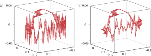
Figure 2. The domain Ω. The convergence history of (PCGM) and (CGM) for both experiences.

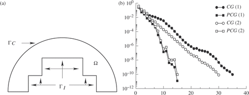
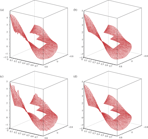
The mesh, displayed in Figure 2(a), has 1283 degrees of freedom with 81 nodes located on Γ_C and as many nodes lie in Γ_I. The exact Cauchy data are polluted by a multiplicative random noise of maximum (relative) magnitude of 10%. The regularization parameters are fixed close to the optimal values for both examples. We mean that the deblurring of the noise is the most efficient for those values. Convergence curves for (CGM) and (PCGM) are provided in Figure 2(b). Numerical evidence show a significant improvement of the convergence due to the preconditioner described in Section 3. Moreover, the plots in Figure 3(a, c) represent u_D and those of (b, d) are for u_N. The relative error of u_D with respect to the exact solution u is similar to the noise magnitude, 0.1, while u_N is a little closer to u, the gap is indeed close to 0.08. Globally, the error remains of the same order as the noise amplitude. However, the perturbations on the Neumann data have an insignificant impact on the quality of u_N and the pollution that may be brought by the Dirichlet condition, through u_D, is partially filtered (from u_N). Users are well-founded to select u_N as a better approximation than u_D.

Figure 3. The Lavrentiev finite element solutions with a noise of 10%, u_D are to the left and u_N to right. The Lavrentiev parameters are selected so as to obtain optimal computations. Upper curves are when Γ_C is the T boundary and lower ones are for the circular boundary playing the role Γ_C. Note that the noise on the Neumann boundary the data has an insignificant effect on u_N, it looks more regular than u_D which suffers from the contamination with the Dirichlet data.

About the regularization parameters. The aim that we have been assigned is to find the role of the regularizing parameter ϱ in the computations. It has to be carefully chosen. The discrepancy principle is liable to predict a near optimal value, the one to balance the accuracy and the stability. To be effective, this principle requires the estimation of the gap intensity ε′ in (23). This preprocessing step has to be realized specifically for each domain. Hereafter, we term by noise level the relative maximum of the perturbations affecting the data (g_h, ϕ_h) During the experimentations, the noise is generated using the Fortran rand function with a uniform density. We take back one of the examples used above where the Cauchy boundary conditions are enforced on the T-portion. The data are disturbed by noises with respective levels 10% and 5%. Several computations are run for different values of ϱ. Table 1 provides the parameters chosen when the Cauchy problem is solved by the Lavrentiev finite element method and the discrepancy principle is used. In the discrepancy principle, σ in (23) is set to 1.05. The optimal column indicates in parentheses the (optimal) parameter ϱ_*; the gap between the (computed, exact) solutions has the lowest max-norm. The results show that the discrepancy principle is capable of providing satisfactory values of the regularization parameter in the finite element context for the data completion problem. Before closing the discussion, we cannot help remarking that the choice σ = 1 in the (DP) brings about some improvement in the quality of the approximation. The results displayed in the last column does not need any further comments. Recall that it is necessary for σ to be greater than one to obtain convergence proofs.

Table 1. The relative error between the computed solution u_N and the exact solution u on the whole domain. The regularization method is either the Lavrentiev or the PCG(NR) method. The parameters ϱ_* and k_* in parenthesis are chosen by means of the discrepancy principle.

	Optimal	DP (σ = 1.05)	DP (σ = 1.0)
Lavrentiev (5%)	(0.003) 0.025	(0.005) 0.033	(0.0025) 0.027
PCG(NR) (5%)	(7) 0.013	(5) 0.047	(7) 0.013
Lavrentiev (10%)	(0.005) 0.039	(0.01) 0.064	(0.005) 0.039
PCG(NR) (10%)	(7) 0.022	(5) 0.055	(6) 0.031
CG(NR) (10%)	(7) 0.47

We now switch to the investigation of the method PCG(NR) as a regularization procedure by itself. An early interruption of the iterating process generates inaccuracy whereas a late stopping of it causes instability. The discrepancy principle is there to select an acceptable stopping iteration k_*. The corresponding rows in Table 1 illustrate the reliability of the method as a regularization strategy, when combined with either of the selection rules. At last, the row CG(NR) in Table 1 is supplied to demonstrate the necessity of the preconditioning. The non-preconditioned (CG) without any supplementary regularization completely fails in achieving acceptable results.

About complex shaped domains. The tests we are concerned with here are motivated by the numerical work on the electrical activity of the brain from Electro-Encephalo-Graphs (EEG). For instance, epileptic focii in the brain cortex may be modelled by dipolar sources and an algebraic technique is proposed in 45 to recover these point-wise sources (see also 46). Roughly said, the potential is recorded at the surface of the scalp, according to a well-established protocol. Cauchy conditions on the scalp are thus available and we may be interested in obtaining the potential at the interface of the brain cortex. To proceed with the algebraic method, entries of a particular matrix should be calculated through integrals that require to handle some data completion problems. In one, we intend to recover the electrical potential at the surface of the cortex from measures picked up on the scalp. The data which may therefore be polluted are inexact. The other, required by the methodology of the detection process 45, is involved in Cauchy conditions fixed on the internal boundary. They are exact and come from harmonic polynomials.

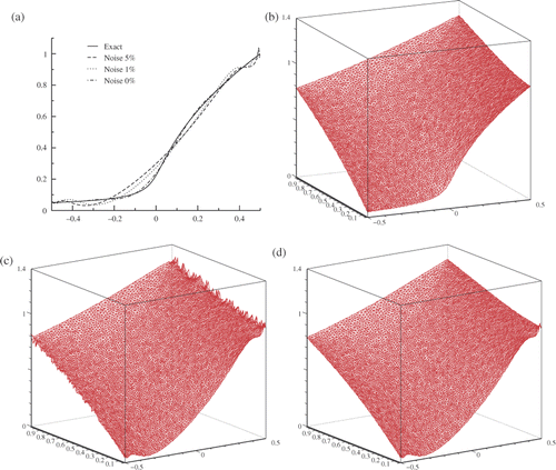
We conduct some computations on the domain of Figure 4 which recall the shape of the external layer of a brain slice. In the first simulations, the internal interface is the Cauchy boundary while the external one is the incomplete boundary. The mesh, constructed from 200 nodes on Γ_I and as many located on Γ_C, is quasi-uniform. In Table 2, we display the relative error of the Lav.-FE and the PCG-FE solutions when the exact solution of the Cauchy problem coincides with some harmonic polynomials. Two cases are considered, either the Cauchy data are exact or contaminated by 5% noise. The regularization parameter ϱ_* for the Lavrentiev regularization and k_* for the PCG regularization are fixed by means of the discrepancy principle with σ = 1. The accuracy obtained by both methods seems satisfactory. The distribution of relative gaps between u_D and u and between u_N and u are plotted in Figure 4 for the solution in the last column of Table 2.

Figure 4. The mesh used (upper panel). The gap between the computed u_D and u (to the left) and between u_N and u (to the right).

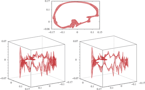
Table 2. The relative error between the computed and the exact solutions. The regularization method is either the Lavrentiev or the PCG(NR) method.

u	xy	x^2 − y^2	x^3 − 3xy^2	−3x^2y + y^3
Lavrentiev (0%)	0.028	0.039	0.031	0.039
PCG(NR) (0%)	0.028	0.038	0.031	0.036
Lavrentiev (5%)	0.074	0.080	0.079	0.073
PCG(NR) (5%)	0.043	0.074	0.080	0.070

The Cauchy problem we investigate in what follows is set on the same domain, but the external boundary is split into a Neumann boundary Γ_N (almost the lower half) and a Cauchy boundary Γ_C. We try to complete the data along the internal interface Γ_I. The context here is different from the previous experiences. Somehow, a fraction of Γ_I lies far away from Γ_C which may be source of more complication. We consider the case where the solution coincides with the one in (25). The Cauchy data on Γ_C so as the Neumann data on Γ_N are polluted by a noise with a 5% intensity. The gap between the exact solution u and the computed ones u_D and u_N is depicted in Figure 5. They look to be a fairly satisfactory approximation of u. The error is close to its maximum in the part bordered by Γ_N which was somehow in agreement with the intuition. Let us finally remark that the optimal parameter ϱ_* is chosen by the discrepancy principle with σ = 1 and depends weakly on the mesh size provided that it is reasonably small. For instance, when 160 nodes are located on Γ_I and 80 nodes on Γ_N, we run computations with 120, 160 or 200 nodes on Γ_C, the value of ϱ_* remains close to 0.25. The error on the exact solution is, respectively, measured to 0.056, 0.052 and 0.062.

Figure 5. The distance to the exact solution of the Lavrentiev finite element solutions. (a) u_D and (b) u_N. The error is maximum at the vicinity of Γ_N. Even though u_N appears les perturbed than u_D, the maximum of the error is similar for both solutions.

About a non-smooth solution. We are involved here in another challenging issue when the data we intend to recover along Γ_I are not smooth. We consider the domain Ω = ]−0.5, 0.5[ × ]0.05, 1[. The Cauchy boundary is the union of the vertical wall Γ_C = {−0.5, 0.5} × ]0.05, 1[, the upper boundary is submitted to a Neumann condition, Γ_N = ]−0.5, 0.5[ × {1} and the lower wall is the incomplete boundary Γ_I = [−0.5, 0.5] × {0.05}. The aim is the finite-element reconstruction of the solution That solution is related to the singularity arisen at the vicinity of a horizontal crack with the tip located at the origin. That singular point is narrowly close to Γ_I, the reconstruction of may therefore suffer from that proximity. We expect that somehow our solver will smooth the computed solution at the middle of Γ_I. As a matter of fact, that is what we observe in Figure 6 where a noise of different magnitudes (0%, 1%, 5%) is affecting the exact Cauchy data. Besides the noise seems to be particularly altering the computed solution at the vicinity of that right extreme-point. The explanation would be the following. Near the incomplete boundary Γ_I, the intensity of the noise may reach its maximal value along the right vertical wall. The peak is actually attained at, respectively, 0.01 and 0.05 for both experiences. At the vicinity of the opposite extreme-point the noise is too small to have a significant effect on the accuracy. This said, apart from the case where no noise is polluting the Cauchy data, the error is maximum at the middle of the edge Γ_I, the nearest point to the singularity. Note that for both noisy computations the relative error for the global solution on the whole computational domain is 0.045 and 0.058, respectively.

Figure 6. Profiles of the exact and computed Lavrentiev solutions along the lower edge, near the singularity (a). The exact solution u (b) and the computed solutions u_D and u_N on the whole domain (c, d).

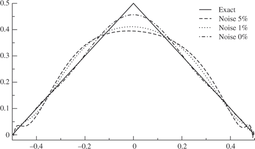
The last numerical experience is concerned with a singularity located this time at the middle of the incomplete boundary Γ_I. The exact unknown data is Obviously λ(·, 0.05) is not differentiable at x = 0. Cauchy data are not known and have to be synthesized. We begin by computing the solution u of a direct problem where the Dirichlet condition on Γ_I is provided by λ and the Neumann condition on the remaining three edges is given by ϕ = 0.5. We consider then the Cauchy problem verified by u. We dispose hence of the Dirichlet condition g = u on Γ_C so that the Cauchy conditions are both available which can be possibly contaminated by adding artificial numerical noises of fixed levels. Once, the data completion problem solved by the Lavrentiev finite element method to obtain u_N (and u_D), the accuracy assessment is made with respect to the reference solution u. The methodology is reasonable enough to resist any contest since we can not claim to have a more accurate solution by handling the ill-posed data completion than by solving the well-posed direct problem. In addition to the dampening of the noise the method is expected to smooth the obtain solution at the vicinity of the angular point (0.5, 0.05). Figure 7 provides the plots of the solution along the incomplete boundary edge. Here again, the maximum of the error is located near the singular point, though it is of satisfactory level. Note that here, the Lavrentiev method is used while for the previous test (PCGM) is employed. In both examples, we operate the discrepancy principle, with σ = 1, for the determination of the regularization parameters k_* and ϱ_*.

Figure 7. Profiles of the exact and computed Lavrentiev solutions along the lower edge. As expected, the maximum of the error is localized near x = 0.5.

7. Conclusion

Computing a reliable solution of the data completion problem is far from being an easy task no matter what the approach used is. The reason lies in the exponential ill-posedness which yields polluting oscillations of the solution unless some suitable regularizing artifices are called for to assure stability. The focus of this article is axed on the approximation of the variational formulation of 24, based on the duplication of the Cauchy solution and relies on the uniqueness Holmgren theorem. We consider and study a discretization by the finite element method which results in a squared, symmetric and non-negative algebraic problem. These properties brings a substantial practical facilities and enable us to use the Lavrentiev method which is the simplest regularization method to dampen the noises that possibly affect the Cauchy data. That Lavrentiev's method shows a similar behavior to Tikhonov's method is somewhat unexpected. The reason is that the discrete problem has a least-square form which may be viewed as the normal equation of some underlying problem. Many of the a posteriori selection rules of the regularization parameter may therefore be explored and the overall analysis conducted in the linear algebra of ill-posed problems are extended as well to our discrete problem. A numerical investigation through multiple examples support the reliability of the Lavrentiev finite element solution associated to the Morozov discrepancy principle. Let us mention before ending that the theoretical counterpart to this work is highly challenging. This consists in stating the convergence proofs of the regularized discrete solution, computed from noisy data, toward the exact solution.

Acknowledgements

This work was partially supported by la region Picardie, programme Appui à l'émergence for Duc Thang Du and by le Ministère de l'Enseignement Supérieur, de la Recherche Scientifique et de la Technologie (MESRST, TUNISIA) under the LR99ES-20 contract for Faten Jelassi.

Notes

Notes

1. The data vector of the auxiliary equation.

2. The choice of (g_h, ϕ_h) should be made so that they converge towards (g, ϕ) in H^1/2(Γ_C) × H^−1/2(Γ_C) which is supposed to be true henceforth.

3. A modern version of Holmgren's theorem, based on Carleman estimates 47, allows us to check that, at the continuous level, the solution u of problem (1–3) is the one whose trace satisfies the fluxes equality a∂_nu_D(λ, g) = a∂_nu_N(λ, ϕ). Actually, the variational problem (7) given later on is related to this fluxes equation.

4. Recall that v_D,h(μ) ∈ X_h,I implies that .

5. We will not make this assumption subsequently.

6. The authors checked that this scheme is nothing other than the algorithm introduced and studied in 18.

7. It may be the case under the discrete uniqueness Holmgren assumption (10).

8. This is equivalent to choosing μ = λ and then μ = λ.

9. They are related to a discrete Holmgren uniqueness assumption on Γ_I similar to (10) where the roles of and are permuted.

10. Using the norm ‖·‖_h indicates that we should rather consider the non-preconditioned problem (12).

11. Computations are achieved on triangular meshes generated by the EMC2 public software (see 48 for the user's guide). The finite elements are linear. The primary procedures, in Fortran 77, are provided in 49. The (CG) and (PCG) inversions of the algebraic equations is achieved by means of a Fortran software downloaded from the CERFACS website 50.

Appendix

The objective here is to show the statement (8) used in the proof of Lemma 2.1. Let us, for convenience, consider the Kohn–Vogelius functional The following result holds.

Lemma A.1

We have that

Proof

We proceed following the lines of 24, Lemma 4.3]. Let us first establish that ∇J_h(·) and ∇K_h(·) coincide. Both gradients can be directly computed. The gradient of J_h(·) is provided as Now, consider Equation (5) for u_N(μ) where ϕ_h = 0, we have that (26) Noting that, due to , there comes out that u_N,h(ϕ_h) ∈ X_h,I. This leads to Back to the gradient of J_h(·), we come up with the final formula The gradient of K_h(·) is given by Observing that implies that (u_D,h(μ) − u_N,h(μ)) ∈ X_h,I. Taking it as a test function in (5) yields that Given that (u_D,h(λ, g_h) − u_N,h(λ, ϕ_h)) ∈ X_h,I, using it as a test-function in (26) we obtain that Substituting in the expression of ∇K_h(·) results in equality ∇J_h(·) = ∇K_h(·). Hence, J_h(·) and K_h(·) differ by an additive constant. The result of the Lemma is completed after remarking that J_h(0) = 0.▪

References

- Andrieux, S, Baranger, T, and Ben Abda, A, 2006. Solving Cauchy problems by minimizing an energy-like functional, Inverse Probl. 22 (2006), pp. 115–134.
- Eldén, L, and Simoncini, V, 2009. A numerical solution of a Cauchy problem for an elliptic equation by Krylov subspaces, Inverse Probl. 25 (2009), Article ID 065002 (22pp).
- Berntsson, F, and Eldén., L, 2001. Numerical solution of a Cauchy problem for the Laplace equation Inverse Probl. 17 (2001), pp. 839–853.
- Leitão, A, 2000. An iterative method for solving elliptic Cauchy problem, Numer. Funct. Anal. Optim 21 (2000), pp. 715–742.
- Tautenhahn, U, 1996. Optimal stable solution of Cauchy problems for elliptic equations, J. Anal. Appl. 15 (1996), pp. 961–984.
- Jourhmane, M, and Nachaoui, A, 2002. Convergence of an alternating method to solve the Cauchy problem for Poisson's equation, Appl. Anal. 81 (2002), pp. 1065–1083.
- Wei, T, Hon, YC, and Ling, L, 2007. Method of fundamental solutions with regularization techniques for Cauchy problems of elliptic operators, Eng. Anal. Boundary Elements 31 (2007), pp. 373–385.
- Cao, H, and Pereverzev, SV, 2007. The balancing principle for the regularization of elliptic Cauchy problems, Inverse Probl. 23 (2007), pp. 1943–1961.
- Cimetière, A, Delvare, F, Jaoua, M, and Pons, F, 2001. Solution of the Cauchy problem using iterated Tikhonov regularization, Inverse Probl. 17 (2001), pp. 553–570.
- Delvare, F, and Cimetière, A, 2008. A first order method for the Cauchy problem for the Laplace equation using BEM, Comput. Mech. 41 (2008), pp. 789–796.
- Ben Abdallah, J, 2007. A conjugate gradient type method for the Steklov–Poincaré formulation of the Cauchy–Poisson problem, Int. J. Appl. Math. 3 (2007), pp. 27–40.
- Johansson, T, 2004. An iterative procedure for solving a Cauchy problem for second order elliptic equations, Math. Nachr. 272 (2004), pp. 46–54.
- Shigeta, T, and Young, DL, 2009. Method of fundamental solutions with optimal regularization techniques for the Cauchy problem of the Laplace equation with singular points, J. Comput. Phys. 228 (2009), pp. 1903–1915.
- Andrieux, S, and Baranger, T, 2008. An optimization approach for the Cauchy problem in linear elasticity, Struct. Multidisc. Optim. 35 (2008), pp. 141–152.
- Hào, DN, Duc, NV, and Lesnic, D, 2009. A non-local boundary value problem method for the Cauchy problem for elliptic equations, Inverse Probl. 25 (2009), p. 055002, (27pp).
- Jin, B, and Zou, Y, 2008. A Bayesian inference approach to the ill-posed Cauchy problem of steady-state heat conduction, Int. J. Numer. Meth. Eng. 76 (2008), pp. 521–3544.
- Ling, L, and Takeuchi, T, 2008. Boundary control for inverse Cauchy problems of the Laplace equations, Comput. Model. Eng. Sci. 29 (2008), pp. 45–54.
- Kozlov, VA, Maz'ya, VG, and Fomin, AV, 1991. An iterative method for solving the Cauchy problem for elliptic equations Comput, Meth. Math.Phys. 31 (1991), pp. 45–52.
- Engl, HW, and Leitão, A, 2001. A Mann iterative regularization method for elliptic Cauchy problems, Numer. Funct. Anal. Optim. 22 (2001), pp. 861–884.
- Cheng, J, Hon, YC, Wei, T, and Yamamoto, M, 2001. Numerical computation of a Cauchy problem for Laplace's equation, ZAMM 81 (2001), pp. 665–674.
- Qian, Z, Fu, C-L, and Xiong, X-T, 2006. Fourth-order modified method for the Cauchy problem for the Laplace equation, J. Comput. Appl. Math. 192 (2006), pp. 205–218.
- Cao, H, Klibanov, MV, and Pereverzev, SV, 2009. A Carleman estimate and the balancing principle in the quasi-reversibility method for solving the Cauchy problem for the Laplace equation, Inverse Probl. 25 (2009), p. 035005.
- Bourgeois, L, 2006. Convergence rates for the quasi-reversibility method to solve the Cauchy problem for Laplace's equation, Inverse Probl. 22 (2006), pp. 413–430.
- Ben Belgacem, F, and El Fekih, H, 2005. On Cauchy's problem I. A variational Steklov–Poincaré theory, Inverse Probl. 21 (2005), pp. 1915–1936.
- Azaïez, M, Ben Belgacem, F, and El Fekih, H, 2006. On Cauchy's problem. II. Completion, regularization and approximation, Inverse Probl. 22 (2006), pp. 1307–1336.
- Groetsch, GW, and Guacaneme, J, 1987. Arcangeli's Method for Fredholm equations of the first kind, Proc. Am. Math. Soc. 99 (1987), pp. 256–260.
- Bakushinsky, A, and Goncharsky, A, 1994. Ill-posed Problems: Theory and Applications. Dordrecht, The Netherlands: Kluwer Academic; 1994.
- Adams, DA, 1975. Sobolev Spaces. New York: Academic Press; 1975.
- Hanke, M, 1995. "Conjugate Gradient type Methods for Ill-posed Problems". In: Pitman Research Notes in Mathematics Series. Vol. 327. Harlow: Longman Scientific and Technical; 1995.
- Ben Belgacem, F, 2007. Why is the Cauchy's problem severely ill-posed?, Inverse Probl. 23 (2007), pp. 823–836.
- Ciarlet, P-G, 1978. The Finite Element Method for Elliptic Problems. Amsterdam: North Holland; 1978.
- Lucht, W, A finite element method for an ill-posed problem, Seventh conference on the numerical treatment of differential equations (Halle, 1994), Appl. Numer. Math. 18 (1995), pp. 253–266.
- Quarteroni, A, and Valli, A, 1999. Domain Decomposition Methods for Partial Differential Equations. Oxford: Oxford University Press; 1999.
- Ben Belgacem, F, El Fekih, H, and Jelassi, F, 2008. The Lavrentiev regularization of the data completion problem, Inverse Probl. 24 (2008), p. 045009, (14pp).
- Du, DT, and Jelassi, F, A preconditioned Richardson's regularization for the data completion problem and the Kozlov–Maz'ya–Fomin method ARIMA, (accepted).
- Ben Belgacem, F, and Kaber, S-M, 2008. Quadratic optimization in ill-posed problems, Inverse Probl. 24 (2008), Article ID 055002 (15pp).
- Hager, WW, 2000. Iterative methods for nearly singular linear systems, SIAM J. Sci. Comput. 22 (2000), pp. 747–766.
- Lavrentiev, MM, 1967. Some Improperly Posed Problems of Mathematical Physics.. New York: Springer-Verlag; 1967.
- Engl, HW, Hanke, M, and Neubauer, A, 1996. "Regularization of Inverse Probl.". In: Mathematics and its Applications. Vol. 375. Dordrecht, The Netherlands: Kluwer Academic; 1996.
- Tikhonov, AN, and Arsenin, VY, 1977. Solution to Ill-posed Problems. New York: Winston-Wiley; 1977.
- Phillips, DL, 1962. A technique for the numerical solution of certain integral equations of the first kind, J. Assoc. Comput. Mach. 9 (1962), pp. 84–97.
- Morozov, VA, 1966. On the solution of functional equations by the method of regularization, Sov. Math. Dokl. 7 (1966), pp. 414–417.
- Nair, MT, and Tautenhahn, U, 2004. Lavrentiev regularization for linear ill-posed problems under general source conditions, J. Anal. Appl. 23 (2004), pp. 167–185.
- Plato, R, 1998. The method of conjugate residuals for solving the Galerkin equations associated with symmetric positive semidefinite ill-posed problems, SIAM J. Numer. Anal. 35 (1998), pp. 1621–1645.
- El Badia, A, and Farah, M, 2007. Identification of dipole sources in an elliptic equation from boundary measurements: application to the inverse EEG problem, J. Inverse Ill-posed Probl. 14 (2007), pp. 331–353.
- Nara, T, 2008. An algebraic method for identification of dipoles and quadrupoles, Inverse Probl. 24 (2008), Article ID 025010 (19pp).
- Isakov, V, 1998. "Inverse Probl. for Partial Differential Equations". In: Applied Mathematical Sciences. Vol. 127. New York: Springer-Verlag; 1998.
- Saltel, E, and Hecht, F, 1995. EMC2, Un logiciel d'édition de maillage et de contours bidimensionnels. Technical Report No. 118. Rocquencourt, FRANCE: INRIA; 1995.
- Lucquin, B, and Pironeau, O, Introduction to Scientific Computing, (English) Translated from the French by Michel Kern, John Wiley & Sons, Chichester, 1998.
- Frayssé, V, and Giraud, L, 2000. A set of conjugate gradient routines for real and complex arithmetics. CERFACS Technical Report TR/PA/00/47, METEOPOLE Campus, Toulouse; 2000.