Abstract
In this article, we propose an algorithm for identifying a moving boundary in a 2D heat conduction equation without using initial data. The algorithm combines the method of lines and a quasi-reversibility method. The latter replaces the heat equation with a fourth-order partial differential equation, thereby stabilizing the problem. With the regularization parameters chosen suitably, the method can give an accurate approximation to the sought-for moving boundary. Numerical examples show that the proposed method is effective and stable.
1. Introduction
In this article, we consider a moving boundary identification problem in two-dimensional (2D) inverse heat conduction, i.e. identify an unknown time-dependent boundary from the Cauchy data specified on the accessible part of the boundary. Such a kind of problem has important engineering applications in nondestructive testing Citation1–5. To the best of our knowledge theoretical issues and computational algorithms related to a moving boundary identification problem are mostly restricted to 1D models Citation2,Citation6–8. High-dimensional problems are far more difficult, and there are only very few works for 2D and 3D problems Citation1,Citation3,Citation4.
The moving boundary problem is severely ill-posed. That is, the solution, even if it exists, does not depend continuously on the given data. Any small errors in the given data might induce large errors in the solution. Due to the diffusive nature of heat conduction, the temperature response away from the boundary is highly damped and lagged behind with respect to the active input data on the boundary. Thus it is nontrivial to obtain a stable approximate boundary.
Several numerical methods have been developed Citation1,Citation3,Citation4,Citation7,Citation8 for the identification problem. Huang et al. Citation1,Citation3,Citation4 used gradient-based methods together with the boundary element technique for estimating moving boundaries for 2D and 3D transient heat conduction with known initial temperature. In Citation7,Citation8, Wei et al. applied Tikhonov regularization and the method of fundamental solutions to reconstruct a moving boundary from Cauchy data for the 1D heat problem in one layer and multilayer domains, where no initial data is assumed. In Citation2, Fredman employed the method of lines to calculate a moving boundary in 1D heat conduction without using a regularization. Liu and Guerrier Citation6 applied a domain embedding method for estimating the moving boundary in an inverse Stefan problem where the initial temperature should be given. However, in many practical problems, e.g. steel production, the initial temperature is not available due to experimental limitations. Theoretically, Manselli and Vesella proved the continuous dependence of moving boundary on non-characteristic Cauchy data under a priori information without using the initial temperature Citation9, see also Citation10 for related conditional stability estimates with a known initial condition. From Citation9 or Citation8, the uniqueness of moving boundary in 1D case is satisfied.
In this article, we use a quasi-reversibility method to identify a moving boundary for a 2D heat conduction in a bounded domain without using the initial temperature. Numerically, we use the method of lines to solve the modified fourth-order heat problem, and then obtain an approximation to the moving boundary.
The outline of this article is as follows. In Section 2, we formulate the problem and propose a regularization method. In Section 3, we introduce the method of lines. Several numerical experiments are presented in Section 4 to illustrate the effectiveness of the proposed method. Finally, in Section 5, we give some concluding remarks.
2. Formulation of the problem and a regularization method
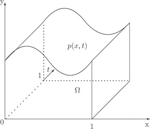
Let Ω = {(x, y, t) ∈ R3|0 < x < 1, 0 < y < p(x, t), 0 < t < 1} be the solution domain, where p(x, t) is an unknown part of the boundary to be determined see for an illustration. The mathematical formulation for a moving boundary problem is given by
(1)
(2)
(3)
(4)
(5)
where u(x, y, t) is the temperature distribution, g1(y, t), g2(y, t), f(x,t) and q(x, t) the given functions satisfying some consistent conditions such as ∂yg1(0, t) = ∂xq(0, t) and so on.
Figure 1. Solution domain.
The boundary identification problem is to determine the unknown boundary function p(x, t) from the Dirichlet boundary condition
(6)
where u0 is a given constant temperature.
It is easy to see that uϵ(x, y, t) = 1 − ϵy + x is a solution for (1) and , uϵ(x, 0, t) = 1 + x and
, the boundary determined by condition (6) with u0 = 0 is
, which tends to infinity as ϵ goes to zero. Thus problem (1–6) is ill-posed in the sense that the boundary does not depend continuously on the input Cauchy data Citation11,Citation12.
Therefore, a regularization method is necessary for stabilizing the problem. In this article, we apply a quasi-reversibility method to construct an approximate solution for problem (1–6). That is, we solve the following problem
(7)
(8)
(9)
(10)
(11)
where α and β are regularization parameters, and
,
, fδ(x, t) and qδ(x, t) are approximate values of g1(y, t), g2(y, t), f(x, t) and q(x, t), respectively. The approximation to the boundary p(x, t) is then determined from the boundary condition
(12)
The quasi-reversibility method was introduced in Citation13, and has been investigated in Citation14–19. The basic idea is to add a higher order derivative term into the partial differential equation so that the original ill-posed problem is transformed into a well-posed one. The idea of adding a second-order derivative in the variable t in a heat equation is due to Weber Citation20. In Citation14, Eldén considered an inverse heat conduction problem by using a quasi-reversibility method. In Citation17, Qian et al. applied a quasi-reversibility method to solve a 2D inverse heat conduction problem and obtained some convergence estimates in which they just used one regularization parameter, i.e. taking α = β in our case (7).
To the best of our knowledge there is no convergence result for this regularization method in the case of a moving boundary identification problem. Also the regularization parameters α and β are generally difficult to choose by an a priori method. Here, we choose the parameters α and β similar to μ in Citation17 by
(13)
where δ is the noise level. If δ = 0, we calculate α and β from (13) with δ = 0.001. Numerical examples in Section 4 show that the computed boundary matches the exact boundary very well. The quasi-reversibility method has an inherent stabilizing effect for noisy input data. Thus our proposed method is feasible and stable.
3. The method of lines
In this section, we use a method of lines to solve the regularized problem (7–11). First, we rewrite Equation (7) in a block operator form with the subscript y denoting the spatial derivative
(14)
and the Cauchy conditions (10), (11) become
(15)
To obtain a numerical solution to problem (14), (15), we apply the method of lines Citation2,Citation21 to discretize equation (14). To this end, we partition the interval [0, 1] into 0 = x0 < x1 < ··· < xN = 1 and 0 = t0 < t1 < ··· < tL = 1, where xi = i · hx, tj = j · τ(i = 0, 1, … , N, j = 0, 1, … , L). Here are
are the step sizes for the space and time variable, respectively.
Next, let vi, j(y) = v(xi, y, tj), M = (N + 1) × (L + 1) and
(16)
where
According to (15), we have
(17)
(18)
where the vectors
and
are given by
,
for i = 0, 1, … , N.
The second-order partial derivative can be approximated by a central difference scheme as
(19)
and
(20)
where (x−1, y, tj) is a ghost point outside the solution domain Ω. According to the Neumann condition (8), by the central difference scheme, we have
(21)
Thus we have
(22)
Inserting (22) into (20), we get
(23)
A similar deduction leads to
(24)
Denote
(25)
where (Vxx)i(y) = [(vxx)i,0(y), (vxx)i,1(y), … , (vxx)i, L(y)]T, i = 0, 1, … , N. Then, from Equations (19), (23) and (24), we have
(26)
where the coefficient matrix Λ ∈ ℝM×M is given by
(27)
in which Λi ∈ ℝ(N+1)×(N+1)(i = 1, 2, 3) is given by
and the vector b1 is given by
(28)
where
Similarly, the second-order partial derivative can be approximated by a central difference scheme as
(29)
Since the initial data is unknown, we use the values at some neighbourhood points to approximate the initial second-order derivative as follows
(30)
A similar deduction leads to
(31)
Denote
(32)
where (Vtt)j(y) = [(vtt)0,j(y), (vtt)1,j(y), … , (vtt)N,j(y)]T, j = 0, 1, … , L. From (29), (30) and (31), we then get
(33)
The coefficient matrix Ψ ∈ ℝM×M is given by
(34)
in which Ψ0 ∈ ℝ(L+1)×(L+1) is given by
The first-order partial derivative can be approximated by the forward difference scheme as
(35)
and
(36)
Similarly, we get
(37)
Denote
(38)
where (Vt)j(y) = [(vt)0,j(y), (vt)1,j(y), … , (vt)N,j(y)]T, j = 0, 1, … , L. From Equations (35), (36) and (37), we have
(39)
where the coefficient matrix Φ ∈ ℝM×M is given by
(40)
in which Φ0 ∈ ℝ(L+1)×(L+1) is given by
With the help of Equations (26), (33) and (39), problem (14) can be discretized into a linear system of ordinary differential equations
(41)
where I is the identity matrix, Λ, Ψ, Φ and b1 are given by (27), (34), (40) and (28), respectively.
Consequently, we get
(42)
where the column vector b is given by
(43)
The Cauchy condition (15) becomes
(44)
There are many feasible methods to solve the system (42–44). In our implementation, we have opted for the forward Euler method, i.e.
(45)
where hy = yk+1 − yk is a step size for the variable y and
From Equations (44) and (45), the temperature distribution in the region y > 0 follows directly.
To determine an approximate boundary, we use a linear interpolation method to find the approximate value of p(xi, tj) for i = 0, 1, … , N, j = 0, 1, … , L. That is, if vi, j(yk) − u0 < 0 and vi, j(yk+1) − u0 > 0, then we choose
.
4. Numerical experiments
In this section we test several examples to demonstrate the feasibility of our approach. The numerical computations are performed using Matlab 6.5.
To check the accuracy of numerical computations, we compute the root mean squares error by the following formula
(46)
The noisy data are generated by
where (g1)i,j, (g2)i, j, fi, j and qi,j are the exact data, rand(i, j) is a random number uniformly distributed in [−1, 1] and the magnitude δ indicates the relative noise level.
4.1. Effect of the regularization method
In this part, we illustrate how regularization improves the accuracy of numerical results. Take an exact solution for problem (1–6) as
(47)
and the moving boundary is given by
for u0 = 0. The boundary data can be calculated from (47). In this example the step size for x is 1/10, for y is 1/9 and for t is 1/10.
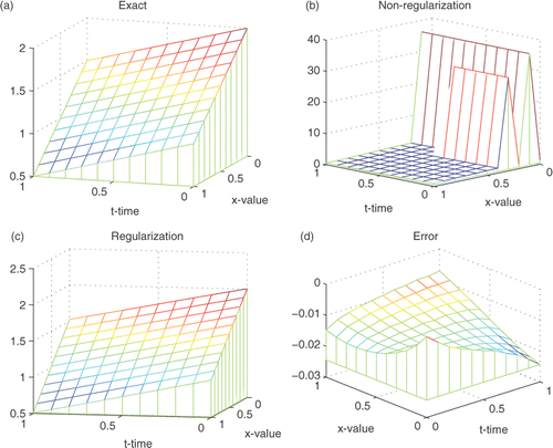
Numerical results for the noise-free data by the our method and a non-regularized method (α = β = 0) are shown in . Observe that the approximation based on regularization agrees well with the exact boundary. In contrast, a stable boundary recovery without using regularization is difficult to obtain. Thus regularization is necessary for stably determining the boundary shape.
Figure 2. (a) The exact boundary; (b) the approximate boundary for δ = 0, α = 0, β = 0, ϵ(p) = 12.203; (c) the approximate boundary for δ = 0.0, α = 0.4343, β = 0.1448, ϵ(p) = 0.0141 and (d) the error between the exact solution and the regularized solution.
The regularization parameters α and β are difficult to determine without a careful convergence analysis. However, motivated by the result in Citation17, we suggest an empirical formula (13) for choosing α and β. We choose various parameters α and β with M = ln(1/0.001), and the respective errors ε(p) are shown in . It is observed that the choice rule (13) gives nearly local minimum error.
Table 1. The root mean square errors for δ = 0.001 with the various parameters α and β where ‘−’ denotes no numerical solution.
4.2. Numerical examples
We test three examples to illustrate the effectiveness of our proposed method.
Example 1
Take an exact solution for problem (1–6) as
(48)
and the steady state boundary p(x, t) = 1 for u0 = 0. In this example the step size for x is 1/15, for y 1/20 and for t 1/15.
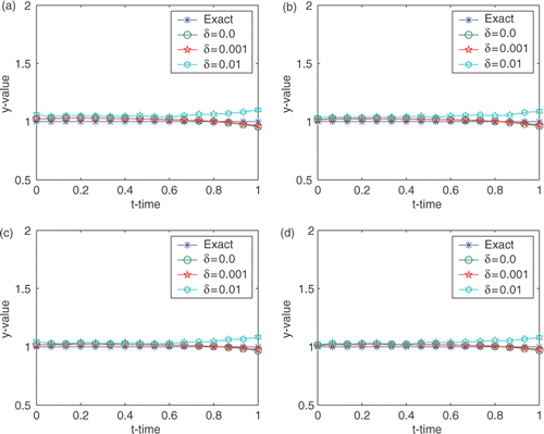
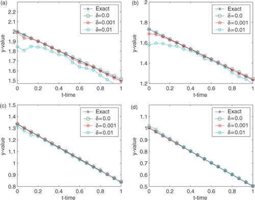
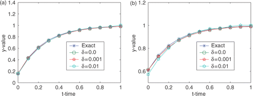
The recovered surfaces for different noisy data are shown in . The curves of
at different positions of x are presented in . We observe that the approximate boundaries match the exact steady state boundary very well. Therefore, our method is stable for small noise levels.
Figure 3. Reconstructed boundary configurations from various noisy data for Example 1. (a) the exact boundary; (b) δ = 0, α = 0.4343, β = 0.1448, ϵ(p) = 0.0201; (c) δ = 0.001, α = 0.4343, β = 0.1448, ϵ(p) = 0.0192; and (d) δ = 0.01, α = 0.6514, β = 0.2171, ϵ(p) = 0.0491.
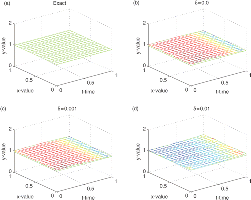
Figure 4. Reconstructed curves at different position of x for Example 1. (a) x = 0; (b) x = 0.2667; (c) x = 0.6667; and (d) x = 1.
Example 2
Take the exact solution for problem (1–6) as
(49)
and the boundary function is given by
for u0 = 0. In this example the step size for x is 1/15, for y is 1/20 and for t is 1/15.
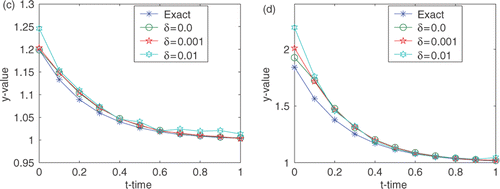
The reconstructed surfaces from different noisy data are shown in . We can see that the smaller the relative noise is, the better the computed approximation is. The curves of
at different positions of x are presented in . The reconstructed boundaries are very accurate compared with the exact one if the noise level is smaller than 1%.
Figure 5. Reconstructed boundary configuration from various noisy data for Example 2. (a) The exact boundary; (b) δ = 0, α = 0.4343, β = 0.1448, ϵ(p) = 0.0061; (c) δ = 0.001, α = 0.4343, β = 0.1448, ϵ(p) = 0.0082; and (d) δ = 0.01, α = 0.6514, β = 0.2171, ϵ(p) = 0.0832.
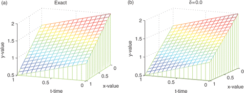
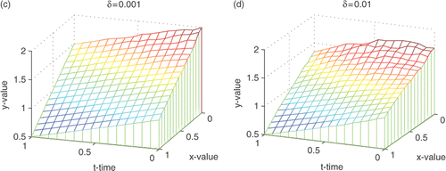
Figure 6. Reconstructed curves at different position of x for Example 2. (a) x = 0; (b) x = 0.2667; (c) x = 0.6667; and (d) x = 1.
Example 3
Take the exact solution for problem (1–6) as
(50)
and the moving boundary is given by p(x, t) = e−4tsin(2x − 1) + 1 for u0 = 0. In this example 3, the step size for x is 1/10, for y 1.8/50 and for t 1/10.
The reconstructed surfaces for different noisy data are shown in . The curves of
at different positions of x are presented in . A good agreement of the approximate boundaries with the exact one is again observed. All numerical results for three examples indicates that our proposed method is feasible and reasonable.
Figure 7. Reconstructed boundary configuration from various noisy data for Example 3. (a) The exact boundary; (b) δ = 0, α = 0.4343, β = 0.1448, ϵ(p) = 0.0284; (c) δ = 0.001, α = 0.4343, β = 0.1448, ϵ(p) = 0.0317; and (d) δ = 0.01, α = 0.6514, β = 0.2171, ϵ(p) = 0.0597.
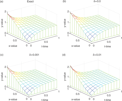
Figure 8. Reconstructed curves at different position of x for Example 3. (a) x = 0; (b) x = 0.3; (c) x = 0.6; and (d) x = 1.
5. Conclusions
In this article, we consider a moving boundary identification problem for 2D heat conduction. The problem is ill-posed in the sense that the solution does not depend continuously on the input data. We use the quasi-reversibility method to transform it into a well-posed one and then use the method of lines to reconstruct a stable approximation of moving boundary. Three examples with various measurement errors are tested. The numerical results show that our method is feasible and stable. Compared with existing methods, it is computationally very efficient, and can handle temporally-spatially dependent boundaries. There are many questions deserving further research. First, the convergence analysis is still missing. Second, a suitable choice rule for the regularization parameters remains unavailable. For real problems, the a priori bound for an unknown solution may not be available, and a posteriori choice methods are of immense interest.
Acknowledgements
This work was supported by the NSF of China (no. 10971089) and the Fundamental Research Funds for the Central Universities (no. lzujbky-2010-k10). The authors would like to thank the referees for their comments and Dr. Bangti Jin for improving our English writing.
References
- Chuang, HC, and Chen, HM, 1999. Inverse geometry problem of identifying growth of boundary shapes in a multiple region domain, Numer. Heat Transfer, Part A. 35 (1999), pp. 435–450.
- Fredman, TP, 2004. A boundary identification method for an inverse heat conduction problem with an application in ironmaking, Heat Mass Transfer (Waerme- und Stoffuebertragung) 41 (2) (2004), pp. 95–103.
- Huang, CH, and Chaing, MT, 2008. A transient three-dimensional inverse geometry problem in estimating the space and time-dependent irregular boundary shapes, Inte. J. Heat Mass Transfer 51 (21–22) (2008), pp. 5238–5246.
- Huang, CH, and Tsai, CC, 1998. A transient inverse two-dimensional geometry problem in estimating time-dependent irregular boundary configurations, Int. J. Heat Mass Transfer 41 (12) (1998), pp. 1707–1718.
- Radmoser, E, and Wincor, R, 1998. Determining the inner contour of a furnace from temperature measurements, Technical Report 12. Linz, Austria: Industrial Mathematics Institute, Johannes Kepler University Linz; 1998.
- Liu, J, and Guerrier, B, 1997. A comparative study of domain embedding methods for regularized solutions of inverse Stefan problems, Int. J. Numer. Meth. Eng. 40 (19) (1997), pp. 3579–3600.
- Wei, T, and Li, YS, 2009. An inverse boundary problem for one-dimensional heat equation with a multilayer domain, Eng. Anal. Boundary Elements 33 (2009), pp. 225–232.
- Wei, T, and Yamamoto, M, 2009. Reconstruction of a moving boundary from Cauchy data in one-dimensional heat equation, Inverse Probl. Sci. Eng. 17 (4) (2009), pp. 551–567.
- Manselli, P, and Vessella, S, 1991. On continuous dependence, on non-characteristic Cauchy data, for level lines of solutions of the heat equation, Forum Math. 3 (5) (1991), pp. 513–521.
- Vessella, S, 2008. Quantitative estimates of unique continuation for parabolic equations, determination of unknown time-varying boundaries and optimal stability estimates, Inverse Probl. 24 (2) (2008), p. 023001.
- Bryan, K, and Caudill, LF, 1998. Stability and reconstruction for an inverse problem for the heat equation, Inverse Probl. 14 (6) (1998), pp. 1429–1453.
- Chapko, R, Kress, R, and Yoon, JR, 1998. On the numerical solution of an inverse boundary value problem for the heat equation, Inverse Probl. 14 (4) (1998), pp. 853–867.
- Lattès, R, and Lions, JL, 1969. "The method of quasi-reversibility. Applications to partial differential equations (Translated from the French edition)". In: Bellman, R, ed. Modern Analytic and Computational Methods in Science and Mathematics. Vol. 18. New York: Elsevier; 1969.
- Eldén, L, 1987. Approximations for a Cauchy problem for the heat equation, Inverse Probl. 3 (2) (1987), pp. 263–273.
- Eldén, L, 1988. Hyperbolic approximations for a Cauchy problem for the heat equation, Inverse Probl. 4 (1) (1988), pp. 59–70.
- Klibanov, MV, and Santosa, F, 1991. A computational quasi-reversibility method for Cauchy problems for Laplace's equation, SIAM J. Appl. Math. 51 (6) (1991), pp. 1653–1675.
- Qian, Z, and Fu, CL, 2007. Regularization strategies for a two-dimensional inverse heat conduction problem, Inverse Probl. 23 (3) (2007), pp. 1053–1068.
- Qian, Z, Fu, CL, and Xiong, XT, 2006. Fourth-order modified method for the Cauchy problem for the Laplace equation, J. Comput. Appl. Math. 192 (2) (2006), pp. 205–218.
- Qian, Z, Fu, CL, and Li, ZP, 2008. Two regularization methods for a Cauchy problem for the Laplace equation, J. Math. Anal. Appl. 338 (1) (2008), pp. 479–489.
- Weber, CF, 1981. Analysis and solution of the ill-posed inverse heat conduction problem, Int. J. Heat Mass Transfer 24 (1981), pp. 1783–1792.
- Berntsson, F, 2002. Boundary identification for an elliptic equation, Inverse Probl. 18 (6) (2002), pp. 1579–1592.