Denoising point cloud

Abstract

A method based on point cloud smoothing approaches for detecting noise and outliers is introduced. This method firstly estimates thresholds according to points’ shifts after smoothing, secondly identifies outliers and noise whose shifts are more than the thresholds and lastly removes them and repeats the whole process. The main difference from other methods is that it tries to screen out outliers from point clouds rather than makes points smoother by correcting their coordinates. The precondition to assure it work is that outliers will be shifted more, which requires smoothing operators possess the ability of low-pass filter. Since this method does not rely on any local parametric representation, it can deal with noisy data in the case of ambiguous orientation and complex geometry. The proposed method is rather simple and can be easily implemented. Some cases are provided to illustrate its feasibility and effectiveness.

Keywords:

• denoising
• smoothing
• point cloud
• low-pass filtering

1. Introduction

To many of the popular research topics in 3D geometry, such as surface reconstruction from unorganized points, and geometry representation with point set instead of mesh, effective and powerful denoising algorithms are of utmost importance 1–4. In general, noise and outliers are related to high frequencies and inliers correspond to the low frequencies in frequency domain. Therefore, devising a low-pass filter is the basic idea of parametrization free smoothing methods, such as λ/μ and Locally Optimal Projection (LOP) operator 5,6. Operators in these low-pass filters are mostly related to the so-called ‘running median’ scheme 7. It is then obvious that high-frequency signals should be farther away from ‘median’ than low-frequency signals. In this sense, the shifts of points in spatial domain provide some evidences for detecting outliers. Considering this fact, our method comes by nature taking smoothing methods as basis.

This article is structured as follows. Section 2 describes the background and related work. Section 3 is devoted to introduce our method. Section 3.3 analyses the density function of transfer function and Section 3.4 gives the rules to choose parameters. In Section 4, we apply our method to some noisy point clouds and compare it with other robust methods. Clean points without obvious shrinkage demonstrate its effectiveness.

2. Related work

In mesh denoising/smoothing, many methods adopt the concept of constrained energy minimization using either the domain of direct neighbours or the global mesh 8. Apart from those surface variational algorithms, other methods remove high-frequency components without relying on the local geometrical information. In the context of unorganized points, there still exist a certain number of methods and most of them are generated from mesh smoothing algorithms 8–17. In this review, we try to include important unorganized points denoising methods and classify them into three kinds: density-based, projection and parametrization free methods.

The density-based method distinguishes clusters and outliers based on the fact that a cluster is the set of all objects which are density-reachable from arbitrary core object in the cluster 18. In other words, for each point in a cluster, its ε-neighbours for some given ε > 0 have to contain a minimum number of points or the density in the ε-ball should exceed a threshold. Therefore, a cluster satisfies two conditions: all points within the cluster are mutually density-connected and if a point is density-connected to any point of a cluster, it belongs to the cluster 19. This character leads to the limitation that it cannot work well when outliers are near to inliers or the density of unorganized points is not uniform.

Projection methods are usually established by defining a consistent geometry for point set 8–15. Levin describes a general method consisting of two steps [16]. Firstly, an approximate hyperplane is determined for each point in a low-dimensional space. This is accomplished by solving a non-linear minimization problem. Then, the hypersurface is interpolated locally by polynomials that have the hyperplanes defined in the first step as domain. To preserve the geometrical feature better, algorithm in 12 is devised by combining Minimum Least Squares (MLS) and the robust statistics method. The basic idea is that a new position of a point is taken as its projection on a local linear plane. The method of average curvature flow is designed on an implicit integration to achieve a robust and scale-dependent Laplacian operator. By deriving a shape operator, principal curvature flow fairing achieves the purpose of enhancing geometric features such as edges and corners when removing noise 11,15. Lange 11 presented a method for anisotropic fairing of a point set based on the concept of anisotropic geometric mean curvature flow. Pauly applied a least-squares optimal Wiener filter for unorganized points after local parametrization and regular resampling 8,11. Hu et al. 8 proposed an anisotropic denoising algorithm by taking the point's normal and curvature as the range component and point's position as the spatial component. Schall et al. 15 developed a local likelihood measure capturing the probability that a 3D point is located on the sampled surface. The likelihood measure is related to the normal directions estimated at the scattered points. Those methods are somewhat feature-preserving, yet their drawback is that results change significantly with the chosen neighbours in the beginning. In addition, their assumption is that the estimated discrete plane can well-approximate the local points. Consequently, they always cannot perform well when noisy data clutters the orientations of points or comprises complex details.

Another kind is the parametrization free method, in sense that it does not rely on estimating normal, fitting a local plane or using any other parametric representation 5,6. It attempts to correct the coordinates to make points smoother rather than to remove outliers from original data. So, it is usually named as the smoothing method. Perhaps the most popular convolution-based smoothing algorithm is the Gaussian filtering method, associated with a scale-space theory. It is well-known that the Gaussian filter can cause obvious shrinkage because Gaussian kernel is not a positively low-pass filter. When it is used, outliers and inliers will converge to the barycentres of all points synchronously. Taking into consideration the problems of volume-shrinkage, the method of λ/μ proposes a strategy of varying scale parameters 5, Desbrun rescales points after each evolution step by the factor of shrinkage, Pauly measures the shrinkage locally and displaces neighbours to compensate the downsized volume 11. Based on Weiszfeld's algorithm for the solution of Fermat–Weber point location problem, LOP removes outliers via a certain fixed-point iteration, where the approximated geometry consists of its stationary points 6. LOP is relatively robust and shows better ability in complex scenarios. However, it still cannot deal with points containing many outliers especially outliers that are concentrated or density-connected with inliers. The main motivation of this article is to overcome this drawback of previous methods.

3. Methodology

3.1. Neighbourhood

Neighbourhood in this article is in the notion of Euclidean vicinity. There are two ways to set the neighbourhood, one is k-nearest neighbourhood and the other is ε-ball neighbourhood. For uniformly distributed points in Euclidean metric, they can obtain similar results. If not, k-neighbourhood may take too far points as neighbours and the radius of ε-ball neighbourhood cannot be reasonably established. So, a compromise strategy is to adopt ε–k-neighbour which is the intersection of k-neighbours with the points contained in ε-ball. In algorithm's implementation, we firstly assign k-neighbours to each point. Then, the radius of ε-ball is estimated by averaging the distances from each point to the farthest point in its neighbours.

3.2. Smoothing transfer function

Since the proposed method takes the parametrization free smoothing method as basis, this section simply analyses the principle of popular smoothing algorithms. In discrete form, the point's shifts can be described by the formula (1) where the weight is positive, is one of the neighbours of and . The weight can be chosen in many different ways by taking neighbourhood structures into consideration. As described in formula (2), a direct and simple strategy with a first-order neighbourhood is to use a positive function defined on the edge. (2)

Intuitionally, the function defined on edge should be some power of edge's length such as and good results may be produced when exponent equals −1. Let be weight matrix with  = 0 when is not in neighbours of . Then, the signal after filtering can be described as (3) is the so-called transfer function of filter. Let matrix be defined as . Formula (3) can be modified as when the smoothing is iterated times. The eigenvalues of matrix , , should be considered as the natural frequencies of the surface, and their corresponding eigenvectors as the associated vibration modes 5. When the transfer function is a type of polynomials, signal can then be decomposed into a linear combination of eigenvectors and eigenvalues as (4)

To define a low-pass filter, a polynomial such that for low frequencies, and for high frequencies in the region of interest should be devised. Gaussian smoothing is a particular case of this definition. It simply sets equal to the inverse of the number of neighbours.

3.3. Density function of point's shift

Since the transfer function will generate different new values for signals with different frequencies, then the function can be taken as the shifts of all points with frequency of . In the case of Gaussian-based polynomials smoothing, the transfer function is defined as . Then, the coordinate shift after times’ iteration is (5)

If and , formula (5) is a monotonic and derivable function. In this situation, the density function of is (6)

If and , the density function of is shown in formula (7). Figure 1 shows the density functions of point's shifts computed using formula (7) with different parameters. (7)

Figure 1. Density function of point's shifts using Gaussian smoothing. For (a)–(d) eigenvalue follows uniform distribution and for (e)–(h) eigenvalue follows norm distribution: (a), (e)  = 0.5,  = 2. (b), (f)  = 0.2,  = 2. (c), (g)  = 0.2,  = 5. (d), (h)  = 0.2,  = 10.

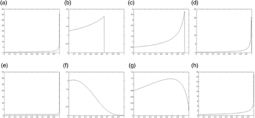
Gaussian kernel is not a low-pass filter kernel according to its Fourier transformation, which can also be found from its density function in Figure 1. After smoothing, the densities of high frequencies are almost same as those of low frequencies, and even higher. The shrinkage in Gaussian smoothing is simply due to the reduction in the low as well as the high-frequency components after repeat iterations.

The method λ/μ intends to provide a non-shrinking algorithm by extending Gaussian kernel to a function defined on surface of arbitrary topology. The corresponding point's shift is (8) where and . Obviously, it is not a monotonic and derivable function in the condition of , then the density functions shown in Figure 2 are estimated using the statistical method.

Figure 2. Density function of point's shifts using the λ/μ method. For (a)–(d) eigenvalue follows uniform distribution and for (e)–(h) eigenvalue follows norm distribution. (a), (e)  = 0.5,  = −0.51,  = 1. (b), (f)  = 0.2,  = −0.21,  = 1. (c), (g)  = 0.2,  = −0.21,  = 5. (d), (h)  = 0.2,  = −0.21,  = 10.

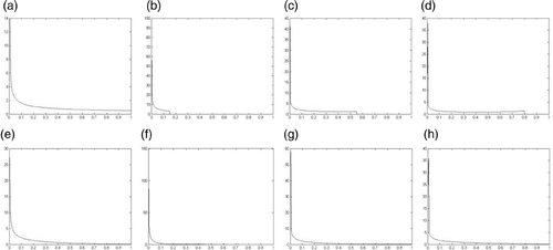
Distribution of is hardly estimated and discussion about the distribution is out of this article's scope. For general situation, we think that follows normal distribution rather than uniform distribution since the high frequencies are relatively less than low frequencies in most of the situations. When filtering high-frequency signals, the method of λ/μ slightly reduces low-frequency signals which can be found in Figure 2, so it still is not a real low-pass operator. However, if high-frequency signals are constantly removed during iterations, low-frequency signals will be filtered with less chance. Therefore, this article devises an iterative algorithm which removes points whose shifts are relatively larger after smoothing. In view of the fact that density function of point's shifts is similar to Gaussian function to great extent, this article approximately uses Gaussian function to describe it.

3.4. Parameter and threshold

According to 5, should be from , should belong to and . When these parameters are in above regions and is in the range of , the function can filter high-frequency signals and control shrinkage. With increasing , point cloud becomes smoother but features cannot be effectively preserved within same iterations. With the difference between and increasing, shrinkage becomes more serious. So, can be considered as controlling smoothing rate and together with is to control shrinkage. We generally suggest that , when point set contains many outliers and , in another situation.

After smoothing, the shifts of all points can be easily obtained and the normal vectors of each point can be estimated with the smoothed points using PCA transformation 1. So, each point's shift along with its normal can be computed. Subsequently, thresholds are established according to Gaussian density function, in which parameters are calculated using formula (9), is the number of points and is one of the point's shifts. (9)

The corresponding threshold can be determined as . We usually set coefficient be from in practical applications. Automatically determining self-adaptive parameters is difficult relying on the potential information of point cloud only.

3.5. Implementation issue

This section describes the complete implementation steps by taking the smoothing method of λ/μ as example.

1.	Establish the k–d tree for point cloud and find the k-neighbours for each point using Approximate Nearest Neighbour (ANN) algorithm.
2.	Compute distance from each point to the farthest point in its neighbours, average these distances to get the radius of ε-ball.
3.	Build ε–k-neighbours for all points: intersect k-neighbours with the points contained in ε-ball.
4.	Apply the λ/μ smoothing method to each point. The weight is defined as , calculate the shifts for each point:

The new position of point will be in odd/even times’ iteration.

1.	Obtain each point's normal by decomposing the matrix

Let , is matrix's eigenvalue and is the associated eigenvector. If , represents the minor direction of neighbours. That means denotes the direction of locally fitted plane. Therefore it can be taken as the normal of current point.

1.	Compute the point's shift along its normal .
2.	Estimate the thresholds as Section 3.4 describes: compute the parameters in Gaussian density function, set the threshold coefficient.
3.	Remove points whose shifts are more than the threshold. If exit condition is satisfied, loop time is over its limitation or no points are removed in recent iteration, break loop.
4.	Return back to step (1).

Complexity of establishing data structure in ANN algorithm is , where represents the number of points in . Finding k-neighbours for all points has complexity. Smoothing process can be done in operations, represents the smoothing times and denotes denoising times. Computation of threshold is a by-product of smoothing. Deleting outliers and noise can be carried out in operations. In total, computation complexity of our method is .

4. Experiment and analysis

In order to evaluate the performance of our algorithm and conduct comparison with other advanced methods, different kinds of noisy data are tested in this experiment. The results show our algorithm can be comparable to those well-known methods and performs better when unorganized points contain many outliers. In quantitative evaluation, only synthetic data are utilized since the standard parameters are always absent for actual data.

4.1. Denoising noisy points

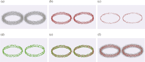
Figures 3 and 4 show the synthetic examples where the correct topology of two near concentric noisy circles and two noisy osculatory cylinders can be obtained using our method. When using LOP, we try to keep points’ distribution as fair as possible 6. For all this, Figure 4(d) still shows serious shrinkage after smoothing. By comparison, the situation is not obvious in Figure 4(b) and the results of our method are comparable to those of LOP and λ/μ.

Figure 3. Denoising 2D noisy data taken from two concentric circles of radii 0.9 and 1.0. The noisy circles are illustrated with black points in (a)–(d). (a) and (b) show the point set after smoothing using λ/μ and LOP, respectively. (c) and (d) show the point set after 1 and 2 iterations using our method. In (e) and (f), green points denote the results of LOP, blue points denote the results using λ/μ and red points show the denoising point set using our method. In (a) and (e), a few remaining floating points still exist and three methods obtain similar results which are robust to noise. Moreover, the shrinkage effect is insignificant for three methods.

Figure 4. Denoising noisy data taken from two osculatory cylinders: (a) two noisy osculatory cylinders, (b) the result after one time's iteration using our method, (c) point set after three iterations using our method, (d) the result of LOP, (e) the combination results of our method and LOP and (f) our result and original point set. Our method shows more robust.

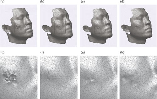
Figure 5 further compares the denoising results using λ/μ, LOP and our method. Detailed features around the eye in Figure 5(b) and (c) are lost, while they are perfectly preserved in Figure 5(d). Moreover, obvious shrinkage appears in Figure 5(b) and (c), which almost can’t be found in Figure 5(d). As the local magnified results show, after removing noise from original data using our method, the noisy region has fewer points than other regions. Then, the difference between our method and others clearly shows that our method is to remove noise while other methods try to correct the coordinates of noisy points. Therefore, we can come to a conclusion that our method is more loyal to the original data and smoothing algorithms obtain smooth results at the expense of accuracy.

Figure 5. Example of denoising a complex point set: (a) the original 3D mesh model of a human face, (b) 3D mesh model after smoothing using λ/μ, (c) 3D mesh model after smoothing using LOP and (d) 3D mesh model after denoising using our method. (e), (f), (g) and (h) are the local magnified regions of (a), (b), (c) and (d), respectively.

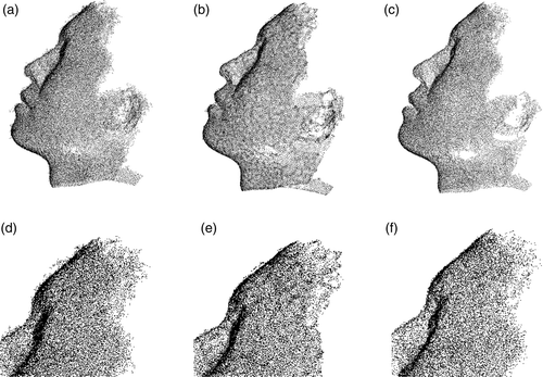
Figure 6(a) shows a point set of a human face which has been processed using Density-Based Spatial Clustering of Applications with Noise (DBSCAN) 7. We can see that there is still a certain amount of noise connected with inliers. Figure 6(b) shows the result after smoothing using λ/μ. It is noticed that all points converge to their barycentres and there are still some outliers near to the mouth and forehead. In smoothing, we set parameters , , and iterative times . Then, we use the points’ shifts to compute the parameters in formula (9) and set thresholds coefficient to obtain the thresholds. After that, points whose shifts are more than threshold are removed and the result is shown in Figure 6(c). Noise and outliers are almost screened out without obvious shrinkage. The total number of points in Figure 6(a) is about 60,000 and that of remaining points in Figure 6(c) is about 50,000.

Figure 6. Raw data set denoising example: (a) a noisy point set, (b) point set after smoothing using λ/μ method and (c) clean data after denoising using our method. (d), (e) and (f) are the local point sets which are corresponding to (a), (b) and (c).

Figure 7(a) shows a point set captured with a 3D human body reconstruction system based on computer stereo vision. Obviously, it has too many outliers and noise. Many outliers are on the equipment of reconstruction system. To date, the quality of original points obtained from this system has been greatly improved, yet this noisy data is still used to test our method. DBSCAN is firstly used to delete parts of outliers, but most of outliers and noise cannot be detected. Using our method, the result after one time's iteration is shown in Figure 7(b). After three time's iterations, a relatively clean data can be obtained as shown in Figure 7(c). Since the original data comprise too many outliers and noise, we set the iterative times to be 35 in smoothing and the coefficient in computing thresholds is . For this data, other methods including λ/μ and LOP cannot produce satisfying results.

Figure 7. Denoising point set comprising a great amount of noise and outliers: (a) original point cloud, (b) result after one time's iteration and (c) result after three time's iterations.

4.2. Quantitative evaluation

Quantitative evaluation on a cylinder's points using the proposed method is conducted to illustrate its robustness. Also, repeat experiments using λ/μ and LOP were provided for comparison. The noisy data is produced by adding Gaussian noise to a synthetic cylinder's points. The number of points is 10,000. Then, denoising is carried out to this noisy data using different methods. Afterwards, we estimate the accuracies of the fitted cylinders which are computed using the points after processing according to least squares rule in all situations. As shown in Table 1, denotes the error of middle axis, is the radius's error and represents the average distance of all points to the fitted cylinder. For λ/μ, radius's error increases after repeat iterations. Similar situation appears in LOP. The reason is that they all cause points shrinkage. So, the radius of fitted cylinder after smoothing becomes smaller. By comparison, our method achieves relative high accuracies because it constantly removes noise and the coordinates of inliers keep unchanged, which means the remaining points are closer to the original cylinder.

Table 1. Evaluation of cylinders’ denoising results.

	Noisy data	λ/μ		Lop		Our method
		50 Iteration	100 Iteration	1 Iteration	10 Iteration	1 Iteration	3 Iteration
	0.06	0.07	0.07	0.03	1.30	0.07	0.03
dR	0.15	0.08	0.13	0.37	0.61	0.04	0.04
dS	3.17	1.95	1.49	0.90	1.01	1.37	0.54

5. Conclusion

After smoothing, all points will converge to their barycentres which are often located in the area with high density. Generally, the coordinate shifts of outliers and noise will be more than those of inliers. According to this principle, a denoising rather than smoothing method has been proposed in this article. The main merit lies in that it can perform well when point set contains much noise and many outliers. Another advantage is that all kinds of smoothing methods possessing low-pass ability can be applied in this method, which expands the scope of its applications. The defects are that it may lead to holes in the regions where noise and outliers are concentrated and parts of inliers may be wrongly removed. For all that, this method is still valuable due to its loyalty to the original data.

Acknowledgements

We acknowledge the valuable comments from the editor and all anonymous reviewers. We would also like to thank the staff working in the Unit of Digital Inspection and Modeling, Industrial Centre, The Hong Kong Polytechnic University for their data and suggestions.

References

- Hoppe, H, Derose, T, Dunchamp, T, Mcdonald, J, and Stuetzle, W, 1994. Surface reconstruction from unorganized points, Comput. Graph 26 (1994), pp. 71–78.
- Peyre, G, and Cohen, L, 2006. Geodesic remeshing using front propagation, Int. J Comput. Vision 69 (2006), pp. 145–156.
- Alexa, M, Behr, J, and Cohen, OD, 2001. Point set surfaces, IEEE Conference on Visualization (2001), pp. 21–28.
- Guennebaud, G, Germann, M, and Gross, M, 2008. Dynamic sampling and rendering of algebraic point set surfaces, Comput. Graph. Forum 27 (2008), pp. 53–662.
- Taubin, G, A signal processing approach to fair surface design, SIGGRAPH’ 95, 1995, pp. 351–358.
- Yaron, L, Daniel, CO, and David, L, 2007. Parameterization-free projection for geometry reconstruction, ACM Trans. Graph 26 (2007), Article No. 22.
- Cheng, Y, 1995. Mean shift, mode seeking, and clustering, PAMI 17 (1995), pp. 190–799.
- Hu, G, Peng, Q, and Forrest, AR, 2006. Mean shift denoising of point-sampled surfaces, Visual Comput 22 (2006), pp. 147–157.
- T.K. Dey, S. Goswami and J. Sun, Smoothing noisy point clouds with Delaunay preprocessing and MLS, Technical Report, Ohio-State University, 2004.
- B. Mederos, L. Velho and L.H. Figueiredo, Robust smoothing of noisy point clouds, SIAM Conference on Geometric Design and Computing, 2003.
- Lange, C, and Polthier, K, 2005. Anisotropic smoothing of point sets, Comput. Aided Geom. D 22 (2005), pp. 680–692.
- Ztireli, AC, Guennebaud, G, and Gross, M, 2009. Feature preserving point set surfaces based on non-linear kernel regression, Comput. Graph. Forum 28 (2009), pp. 493–501.
- U. Clarenz, U. Diewald and M. Rumpf, Anisotropic geometric diffusion in surface processing, Proceedings of the Conference of Visualization, Los Alamitos, CA, 2000, pp. 397–405.
- Liu, Y, Paul, J, Yang, J, Yu, P, Zhang, H, and Sun, J, 2006. Automatic least-squares projection of points onto point clouds with applications in reverse engineering, Comput. Aided Design 38 (2006), pp. 1251–1263.
- O. Schall, A. Belyaev and H.P. Seidel, Robust filtering of noisy scattered point data, Proceedings of Eurographics Symposium on Point-Based Graphics, 2005, pp. 71–77.
- D. Levin, Mesh-independent surface interpolation, in Geometric Modeling for Scientific Visualization, G. Brunnett, H. Müller, B. Hamann and L. Linsen, eds., Springer-Verlag, Berlin Heidelberg, 2003, pp. 37–49.
- Marco, M, Luca, P, Augusto, S, and Stefano, T, 2008. Fast PDE approach to surface reconstruction from large cloud of points, Comput. Vis. Image Und 12 (2008), pp. 274–285.
- M. Ester, H.P. Kriegel and J. Sander, A density-based algorithm for discovering clusters in large spatial databases with noise, Proceedings of 2nd International Conference on Knowledge Discovery and Data Mining, 1996, pp. 226–231.
- P.K. Hans and P. Martin, Density-based clustering of uncertain data, The 11th ACM SIGKDD International Conference on Knowledge Discovery and Data Mining, 2005, pp. 672–677.