Identifying an unknown source term in radial heat conduction

Abstract

In this article, we consider an inverse problem of determining an unknown heat source term from the final temperature history of the radial domain. This problem is ill-posed: the solution (if it exists) does not depend continuously on the final data. A spectral method is applied to formulate a regularized solution and a logarithmic-type error estimate for the regularized solution is given under a suitable choice of regularization parameter. Numerical results are presented to illustrate the accuracy and efficiency of the method. Meanwhile, the uniqueness of solution for the problem is provided.

Keywords:

• ill-posed problem
• heat source
• identification
• spectral method
• error estimate

AMS Subject Classifications::

• 35R25
• 35R30
• 65J20
• 65M30

1. Introduction

Let Ω ∈ ℝ^N be a heat conduction body, T > 0 and u represent the temperature satisfying the following heat equation: (1) where a² is the thermal diffusivity and the right-hand side f denotes a heat source. Unfortunately, the characteristics of source in actual problems are sometimes unknown. There are inverse problems which determine the heat source from the final temperature history or the boundary temperature history.

The inverse heat source problems have extensive application background and important theoretic significance, so the problems have a long development history 1–9. These problems are classical ill-posed problems, and some theories and extremely effective algorithms have been obtained. For instance, uniqueness and conditional stability results can be found in 10.

In recent years, due to taking a more and more important role in migration of groundwater, identification and control of pollution source and environmental protection, inverse heat source problems have been considered by many authors by different methods 11–21. Namely, these have been the mollification method 17,18, iterative regularization methods 19–21, boundary element method 13, the finite difference method 14 and radial basis functions 12. However, the results available in the literature on the inverse heat source problem are mainly devoted to numerical methods. Only a few analytical methods were presented for these problems 22,23. But in most cases the stability theory with explicit error estimate has not been generalized accordingly. In this article, we use a spectral method to deal with an inverse heat source problem in a radially symmetric region and obtain a logarithmic-type error estimate for the regularized solution.

The physical model considered here is an infinitely long cylinder of radius r₀ with given initial temperature, which is considered axisymmetric and the surface temperature distribution is zero. The correspondingly mathematical model of our problem can be described by the following radial heat equation: (2) with the initial condition and final observation at t = T, namely (3) and the boundary conditions (4) where r is the radius. For simplicity, in this article we assume that the initial temperature vanishes. If the initial condition u(r, 0) = h(r) does not vanish, the problem can be divided into a well-posed problem and an ill-posed problem with u(r, 0) = 0.

The inverse heat source problem (1.2–1.4) requires the recovery of pair of functions (u, f). This problem is an ill-posed problem (the details will be given in section 2). Hence, regularization is needed. Prior to this study, Berntsson 24 and Tautenhahn 25 have applied a spectral method to the sideways inverse heat conduction problem. In this article, we will use their spectral method to solve the inverse source problem (1.2–1.4).

This article is organized as follows. In Section 2, the solution of the problem (1.2–1.4) is given. In Section 3, the uniqueness of the solution is provided. Section 4 presents the error estimate for the spectral method. To verify the efficiency and accuracy of the spectral method for problem (1.2–1.4), we give some numerical examples in Section 5.

2. Solution of problem (1.2–1.4)

As a solution of problem (1.2–1.4), we understand a function u(r, t) satisfying (1.2–1.4) in the classical sense and for every fixed r ∈ [0, r₀], the function u(r, ·) ∈ L²[0, T] . In this class of functions, if the solution of problem (1.2–1.4) exists, then it must be unique (the details will be given in Section 3). We denote by L²[0, r₀; r] the Hilbert space of Lebesgue measurable functions f with weight r on [0, r₀]. We denote by (·, ·) and ‖·‖ the inner product and norm on L²[0, r₀; r], respectively, with the norm Assume that u(r, t) is the unique solution of problem (1.2–1.4). Applying the method of separation of variables, we have the following lemma.

Lemma 2.1

If the solution of problem (1.2–1.4) exists, then it is given by (5) where (6) J₀(z) and J₁(z) denote the 0th order and 1st order Bessel functions, respectively 26, and are the sequence of roots of the equation J₀(z) = 0 which satisfy

Proof

Applying the method of separation of variables, we seek a solution of problem (1.2–1.4) with the form (7) Substituting (2.3) into Equation (1.2) and boundary conditions (1.4), we can show that R(r) satisfies the following ordinary differential equation and boundary conditions: (8) (9) where λ is an unknown constant. The eigenvalues of problem (2.4)–(2.5) are and the corresponding eigenfunctions are Thus the solution u(r, t) and nonhomogeneous term f (r) of problem (1.2–1.4) can be represented as follows: (10) (11) where According to the properties of J₀(x), the eigenfunction's system is complete, and orthogonal with weight r on [0, r₀].

Substituting (2.6) and (2.7) into Equation (1.2) and the initial condition in (1.3), we can show that υ_n(t) satisfies Solving this initial problem yields (12) Then, from (2.6) and (2.8) we have From (1.3) at t = T we have (13) From the above formula we can obtain (2.2). This proves the lemma.▪

Since formula (2.9) can be rewritten as (14) Denote by (15) the eigenfunctions system which is orthonormal with weight r on [0, r₀]. It is also a complete system in L²[0, r₀; r]. Using (2.2), (2.7) and (2.11), Equation (2.10) can be rewritten as Then we have and (16)

Since measurement errors exist in g(r), the solution has to be reconstructed from noisy data g_δ(r) which is assumed to satisfy (17) where g(·) and g_δ(·) belong to L²[0, r₀; r].

We also assume that there exists an a priori condition for problem (1.2–1.4): (18) where ‖ f ‖_p is defined by

Applying (2.12) yields (19) Note that μ_n tends to infinity as n tends to infinity. Therefore tends to infinity as n tends to infinity. Formula (2.15) implies a rapid decay of |(g(r), ω_n(r))| for n large enough. But such a decay is not likely to occur in the measured noisy data g_δ(r) at t = T. So, small perturbations of g(r) can blow up and completely destroy the solution f (r), i.e. problem (1.2–1.4) is ill-posed.

3. Uniqueness

Let g be a known function in L²[0, r₀; r]. We consider the problem of identifying a pair (u, f).

Theorem 3.1

Let u_i ∈ C^2,1((0, r₀) × (0, T] ), f_i ∈ L²[0, r₀; r], (i = 1, 2). If (u_i, f_i), (i = 1, 2) satisfy (1.2–1.4), then (u₁, f₁) = (u₂, f₂).

Proof

Put , then satisfy (20) Introduce the function (21) where (22) From (3.1–3.3) we can show that ν(r, t) satisfies the following problem: (23) (24) (25) Using (3.4)–(3.6), we conclude that Therefore, i.e. and thus ν(r₀, t) = C(t). Combining this with (3.5) yields (26) Combining (3.7) with (3.6), we have (27) and (28) By differentiating (3.9) with respect to r, one obtains . Substituting (3.7) and (3.8) into (3.2) yields . Thus the uniqueness is proved.▪

4. Regularization and error estimate

In this section we consider under conditions (2.13) and (2.14) how to stabilize the radial inverse heat source problem (1.2–1.4) in the interval r ∈ (0, r₀) by a spectral method.

A natural way to stabilize the problem is to truncate the series (2.12). Therefore, we introduce a function q given by (29) This function is called a regularizing filter and this choice of q is called the spectral cutoff 27. Then, for any noisy data g_δ which satisfies (2.13) we get a regularized approximate solution : (30) We call it the spectral cutoff solution of problem (1.2–1.4) in the interval 0 < r < r₀. We now give the following results.

Theorem 4.1

Let f (r), given by (2.12), be the exact heat source for r ∈ (0, r₀) and , given by (4.2), be the regularized approximate heat source to f (r). Let the measured data at t = T, g^δ(r), satisfy the condition (2.13) and the a priori condition (2.14) be valid. If we select the regularization parameter α as (31) then the following stability estimate holds: (32)

Proof

From (2.12) and (4.2), we find that According to the properties of the Bessel function J₀(x), there exists a positive constant c such that, for all natural numbers n, (33) Due to (34) we have From conditions (2.13), (2.14) and the choice of α given by (4.3), we find that Note that Thus estimate (4.4) is proved.▪

We can see that estimate (4.4) is a logarithmical stability estimate which is similar to the convergence estimate in 28–30 on the surface.

Remark 4.2

In general, the a priori bound E in (2.14) is not known exactly. In this case, for Theorem 4.1, with we have where E is only a bounded positive constant and it is not necessary to know it exactly.

5. Numerical experiments

In this section, we will describe the numerical implementation of the spectral method, and some numerical results are given to illustrate the effectiveness of the suggested regularization method. For simplicity, we take T = 1 in all the following examples. The number of points on the grid in the space-time domain are taken to be M = K = 31.

For clarity, capital letter represents the samples from function g(·). The noisy data is generated by the function randn given in Matlab, i.e., The function ‘randn(·)’ generates arrays of random numbers whose elements are normally distributed with mean 0 and variance 1. The noise level δ is computed according to Furthermore, in order to present the performance of the spectral method, we will define the relative root mean square error (RRMSE) as where and represent the discrete form of the exact and approximated source, respectively.

From (4.2) we know that Combining (4.1) and Simpson's rule, the above approximation can be written as where N is the positive integer which satisfies and , and

Now we consider the following four examples.

Example 1

The exact solution of problem (1.2–1.4) with g(r) = J₀(r)(1 − e⁻¹) is given by

With the help of Matlab, we get some values of the roots of equation J₀(z) = 0, i.e. μ₁ ≐ 2.4049, μ₂ ≐ 5.5202, μ₃ ≐ 8.6539, μ₄ ≐ 11.7916, μ₅ ≐ 14.9310, μ₆ ≐ 18.0711, μ₇ ≐ 21.2117, μ₈ ≐ 24.3525, etc. According to Remark 4.2, we take the regularization parameter α = 18.9005 with p = 2 and ϵ = 1%. It is obvious that if , we should take N = 1 for Example 1 with ϵ = 1%. In Table 1, the relative errors between the exact source function and the numerical ones corresponding to various N are presented. We can see that the computed source function is best for N = 1 and the result is acceptable for N = 2, 3, 4, 5, i.e. the approximations are not very sensitive to variations of the parameters. From Table 2, we find that M has little influence on the results when it becomes large, so we take M = 31 in the numerical test for this example.

Table 3 lists the influence of p on α with ε = 1% for Example 1. It can be seen that the regularization parameter α corresponding to different p all satisfy . According to the definition of regularization solution, we should take N = 1 for these cases. As p has little influence on the regularization parameter, we always take p = 2 for simplicity.

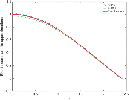
Figure 1 shows the comparison between the exact solution and its approximation with different noise level for Example 1. We can see that with up to 10% noise in the data, the numerical source function is still in good agreement with the exact one.

Sometimes it is difficult to find a pair of functions (u, f) which satisfy the problem (1.2–1.4) simultaneously. For this case, we take a f (r) ∈ L²[0, r₀] and compute the solution of the direct (35) (36) (37) to obtain the final data g(r) = u(r, T). The above-mentioned well-posed problem will be discretized by the standard Crank–Nicholson difference scheme. Now we consider three examples for which there are no analytical solutions available.

Figure 1. The comparison between the exact source function and the numerical ones with N = 1 and p = 2 for various levels of noise in the data, for Example 1.

Table 1. Relative error RRMSE(f) with ϵ = 1%, M = 31 for Example 1.

N	1	2	3	4	5	6	7	8
RRMSE(f)	0.0022	0.0079	0.0261	0.0195	0.0660	0.1948	0.3780	0.3286

Table 2. Relative error RRMSE(f) with ϵ = 1%, N = 1 for Example 1.

M	11	31	51	81	101	201	301	401
RRMSE(f)	0.0091	0.0022	0.0025	0.0024	0.0031	0.0020	0.0020	0.0028

Table 3. The influence of different p on α with ϵ = 1% for Example 1.

p				1	2	3
α	25.9760	25.4262	24.3266	22.1275	18.9005	13.3309

Example 2

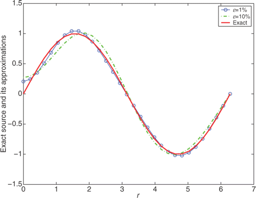
Consider a smooth heat source f (r) = sin(r), 0 ≤ r ≤ 2π.

Example 3

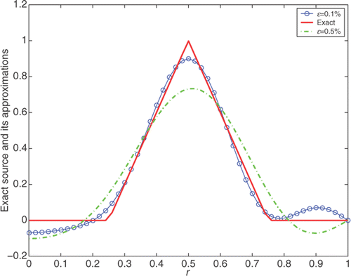
Consider a non-smooth but continuous heat source

Example 4

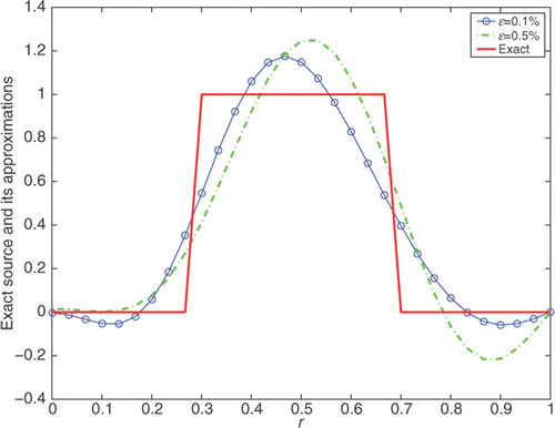
Consider a discontinuous source function

For Examples 2–4, which have no analytic solutions, the data g(r) is obtained by solving the direct problem (5.1–5.3). Because new errors must appear in the computational process, we can appropriately adjust the regularization parameter to obtain a better result. Tables 4–6 list the influence of M on the accuracy of the solution. From these tables, we can see that M has little influence on the results when it is beyond 31 for Examples 2 and 4. While for Example 3, a little could be gained when M is beyond 51. Thus in the following numerical tests we take M = 31 for Example 2 and 4, and take M = 51 for Example 3. Figure 2 illustrates that the numerical results are quite satisfactory for smooth source function, and the smaller the noise, the better the results. Figures 3 and 4 indicate the comparisons between the exact solution and its approximation for non-smooth but continuous and discontinuous case, respectively. The problems with non-smooth solutions generally present great numerical challenge, and it is often difficult to obtain an accurate reconstruction. It can be seen from the two figures that the numerical source functions fail to capture the corner. While taking the ill-posedness into consideration, the numerical results give reasonable approximations.

Figure 2. The comparison between the exact source function and the numerical ones with N = 5, p = 2 for ϵ = 1% and N = 4, p = 2 for ϵ = 10%, for Example 2.

Figure 3. The comparison between the exact source function and the numerical ones with N = 6, p = 2 for ϵ = 0.1% and N = 4, p = 2 for ϵ = 0.5%, for Example 3.

Figure 4. The comparison between the exact source function and the numerical ones with N = 6, p = 2 for ϵ = 0.1% and N = 4, p = 2 for ϵ = 0.5%, for Example 4.

Table 4. Relative error RRMSE(f) with ϵ = 1%, N = 5 for Example 2.

M	11	31	51	81	101	201	301	401
RRMSE(f)	0.2562	0.0874	0.0877	0.0797	0.0668	0.0686	0.0736	0.0746

Table 5. Relative error RRMSE(f) with ϵ = 0.1%, N = 6 for Example 3.

M	11	31	51	81	101	201	301	401
RRMSE(f)	0.5734	0.1465	0.1050	0.0842	0.1054	0.0820	0.0885	0.0898

Table 6. Relative error RRMSE(f) with ϵ = 0.1%, N = 6 for Example 4.

M	11	31	51	81	101	201	301	401
RRMSE(f)	0.5600	0.3277	0.3379	0.3186	0.3209	0.3382	0.3074	0.3175

Acknowledgements

The authors would like to present great thanks to the referees for their valuable comments and suggestions. The work is supported by the National Natural Science Foundation of China (No. 11171136), the Fundamental Research Fund for Natural Science of Education, Department of Henan Province of China (No. 2009B110007), the Hight-level Personnel Fund of Henan University of Technology (No. 2007BS028), the Natural Science Foundation of Henan Province of China (No. 102300410118) and the Natural Science Foundations of Henan University of Technology (No. 10XZP006; No. 09XZZ038).

References

- Cannon, JR, 1968. Determination of an unknown heat source from overspecified boundary data, SIAM J. Numer. Anal. 5 (1968), pp. 275–286.
- Cannon, JR, and Duchateau, P, 1998. Structural identification of an unknown source term in a heat equation, Inverse Probl. 14 (1998), pp. 535–551.
- Cannon, JR, and Esteva, SP, 1986. An inverse problem for the heat equation, Inverse Probl. 2 (1986), pp. 395–403.
- Duchateau, P, and Rundell, W, 1985. Unicity in an inverse problem for an unknown reaction term in a reation–diffusion-equation, J. Differ. Eqns. 59 (1985), pp. 155–164.
- Hettlich, F, and Rundell, W, 2001. Identification of a discontinuous source in the heat equation, Inverse Probl. 17 (2001), pp. 1465–1482.
- Silva Neto, AJ, and Özisik, MN, 1992. Two-dimensional inverse heat conduction problem of estimating the time-varying strength of a line heat source, J. Appl. Phys. 71 (1992), pp. 5375–5362.
- Rundell, W, 1980. Determination of an unknown non-homogeneous term in a linear partial differential equation fromoverspecified boundary data, Appl. Anal. 10 (1980), pp. 231–242.
- Solov'ev, VV, 1990. Solvability of the inverse problem of finding a source, using overdetermination on the upper base for a parabolic equation, Differ. Eqns. 25 (1990), pp. 1114–1119.
- Gol'dman, NL, 2005. Determination of the right-hand side in a quasilinear parabolic equation with a terminal observation, Differ. Eqns. 41 (2005), pp. 384–392.
- Cannon, JR, and Esteva, SP, 1991. Uniqueness and stability of 3D heat source, Inverse Probl. 7 (1991), pp. 57–62.
- Constales, D, Kacur, J, and Van Keer, R, 2002. Parameter identification by a single injection-extraction well, Inverse Probl. 18 (2002), pp. 1605–1620.
- Dehghan, M, and Tatari, M, 2002. Determination of a control parameter in a one-dimensional parabolic equation using the method of radial basis functions, Math. Comput. Model. 8 (2) (2002), pp. 161–168.
- Farcas, A, and Lesnic, D, 2006. The boundary-element method for the determination of a heat source dependent on one variable, J. Eng. Math. 54 (2006), pp. 247–253.
- Fatullayev, AG, 2002. Numerical solution of the inverse problem of determining an unknown source term in a heat equation, Math. Comput. Simul. 8 (2) (2002), pp. 161–168.
- Li, GS, Ma, YC, and Li, KT, 2003. An inverse parabolic problem for nonlinear source term with nonlinear boundary condition, J. Inverse Ill-posed Probl. 11 (4) (2003), pp. 371–387.
- Mahar, PS, and Datta, B, 2001. Optimal identification of ground-water pollution source and parameter estimate, J. Water Res. Plan. Manage. 127 (1) (2001), pp. 20–29.
- Yi, Z, and Murio, DA, 2004. Source term identification in 1-D IHCP, Comput. Math. Appl. 47 (2004), pp. 1921–1933.
- Yi, Z, and Murio, DA, 2004. Source term identification in 2-D IHCP, Comput. Math. Appl. 47 (2004), pp. 1517–1533.
- Johansson, BT, and Lesnic, D, 2007. Determination of a spacewise dependent heat source, J. Comput. Appl. Math. 209 (2007), pp. 66–80.
- Johansson, BT, and Lesnic, D, 2007. A variational method for identifying a spacewise-dependent heat source, IMA J. Appl. Math. 72 (6) (2007), pp. 748–760.
- Johansson, BT, and Lesnic, D, 2008. A procedure for determining a spacewise dependent heat source and the initial temperature, Appl. Anal. 87 (2008), pp. 265–276.
- Choulli, M, and Yamamoto, M, 2004. Conditional stability in determining a heat source, J. Inverse Ill-posed Probl. 12 (3) (2004), pp. 233–243.
- Li, GS, and Tan, YG, 2005. A conditional stability for an inverse problem arising in groundwater pollution, J. Chin. Univ. 14 (3) (2005), pp. 217–225.
- Berntsson, F, 1999. A spectral method for solving the sideways heat equation, Inverse Probl. 15 (1999), pp. 891–906.
- Tautenhahn, U, 1997. Optimal stable approximations for the sideways heat equation, J. Inverse Ill-posed Probl. 5 (1997), pp. 287–307.
- Abramowitz, M, and Stegun, IA, 1972. Handbook of Mathematical Functions. New York: Dover Publications; 1972.
- Kirsch, A, 1996. An Introduction to the Mathematical Theory of Inverse Problems. New York: Springer; 1996.
- Nair, MT, and Tautenhahn, U, 2004. Lavrentiev regularization for linear ill-posed problems under general source conditions, J. Math. Anal. Appl. 23 (1) (2004), pp. 167–185.
- Cheng, W, Fu, CL, and Qian, Z, 2007. A modified Tikhonov regularization method for a spherically symmetric three-dimensional inverse heat conduction problem, Math. Comput. Simul. 75 (3–4) (2007), pp. 97–112.
- Cheng, W, and Fu, CL, 2009. Two regularization methods for an axisymmetric inverse heat conduction problem, J. Inverse Ill-posed Probl. 17 (2) (2009), pp. 159–172.