Estimation of temperature between plates of different footprints by an iterative approach

Abstract

In an electronic cooling application, it is possible to have solid blocks of different sizes attached together in order to spread heat leaving a die. Also, there are other applications where there is heat transfer between two bodies of different dimensions. Here, we consider a simplified model mainly to study the performance of iterative analytical/numerical solutions to these problems. The analytical procedure leads to an integral equation. Then, the heat flux and temperature at the interface are computed using an iterative technique. To verify the accuracy, selected data are compared with numerically determined values. Although, the presented computational procedure is for a two-dimensional solution, the methodology applies equally to three-dimensional problems.

Keywords:

• electronic cooling
• heat spreader
• iterative technique
• integral equation
• heat conduction

Nomenclature

a, b	=	dimensions of Plate 1, see Figure 1
An,	=	constants in Fourier series, Equation (4)
c, d	=	dimensions of Plate 2, see Figure 1
Bi	=	Biot number hc/k2
Bn Cn,	=	constants in Fourier series, Equations (10) and (16)
kj	=	thermal conductivity in Layer j, W m−1 K−1
m, n	=	indices
q0	=	heat flux at y = 0, W m−2
qw	=	input wall heat flux, W m−2
T0	=	reduced temperature at y = 0, K
Tj	=	reduced temperature in Layer j, K
x, y, z	=	coordinates, m

Greek

ε	=	spacing between y and axes in Figure 1
ζ	=	coordinate parallel to z-direction
	=	coordinate parallel to y-direction
	=	physical temperature, K
θ∞	=	temperature of surroundings, K
ξ	=	coordinate parallel to x-direction
ω	=	relaxation factor

Subscripts

m, n	=	indices
w	=	wall condition at y = b
x, y, z	=	coordinate directions

1. Introduction

The thermal performance of microprocessors is an important issue in manufacturing of the electronic devices. A typical high-end microprocessor is comprised of an integration of different functional components such as level two (L2) cache memory, high-speed I/O interfaces and memory controller. In this architecture, certain functional units on the microprocessor dissipate a significant fraction of the total power while others dissipate little or no power. This highly non-uniform power distribution results in a large temperature gradient with localized hot spots that may have detrimental effects on computer performance, product reliability and yield. This processor is then packaged as a first-level module to the rest of the system. The module consists of different materials with varying footprints such as thermal interface material, spreader and heat sink. The resulting spreading resistance can be quite significant and as such it is important to understand the heat transfer process for a potential multi-objective optimization that takes into effect both the heat transfer and architecture performance.

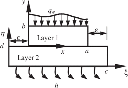
The adequate cooling improves the corresponding speed of data execution. Numerical and theoretical study as to determination of the thermal performance is available in the literature. The related information and adequate citation are in 1–5. The analytical determination of the temperature field in a two-layer system, as shown in Figure 1, is the objective of this presentation. This type of system can appear in different engineering applications such as electronic cooling devices. The Plate 1, Layer 1 in Figure 1, can be viewed as a die with non-uniform power distribution. The Plate 2, Layer 2 in Figure 1, can be viewed to as a heat spreader connected to a heat sink. Numerical studies to the related problems are given in 6, which also contain details related to these types of devices.

Figure 1. Schematic representation of a two-layer body and the coordinates.

The objective of this study is to examine a suitable iterative procedure for a relatively accurate determination of the temperature field in a multi-layer domain, as shown in Figure 1. In practice, each of the Layers 1 and 2 may contain two or more layers. However, for convenience of the presentation of this iterative procedure, Layers 1 and 2 are selected to be a single layer as depicted in Figure 1. Additionally, the mathematical steps are presented for a two-dimensional case. The extension to three-dimensional case requires a minor modification although the equations become a bit lengthy. In general, the mathematical procedure leads toward an integral equation to be solved by an iterative technique. The mathematical procedure leads to a system of two integral equations with two unknowns. Although, this is a well-posed problem, the solution technique is similar to those observed for inverse problems. Classical description of various inverse techniques is well documented in 7–10. As an illustration, the function specification and other techniques have been used to solve transient and steady state inverse heat conduction problems by many investigators (see, e.g. 11–16). In this presentation, an iterative inverse procedure is selected for estimation of the temperature field and this becomes equivalent to the function specification method. For this well-posed problem, an iterative procedure using function specification method 11,12 is selected for estimation of the temperature field.

2. Mathematical relations

The analytical determination of the temperature field within a two-layer body, when each layer has a different size, is the subject of the following formulations. The schematic representation of the regions and the coordinate systems are shown in Figure 1. The governing equations for the steady state heat conduction satisfy the Laplace equations (1) with j = 1 in Layer 1 and j = 2 in Layer 2. In this analysis, the function represents the reduced temperature so that ; where is the physical temperature and is the temperature of the surroundings. We conside the insulated boundary conditions in x- and z-directions. Therefore, for the convenience of properly demonstrating this presentation, a two-dimensional case is selected within the subsequent mathematical presentations. An extension of this mathematical technique to three-dimensional problems is discussed in a later section.

Clearly, there are two temperature solutions: one for Layer 1 and the other for Layer 2. These two solutions must satisfy the boundary conditions and the compatibility conditions between the two layers.

2.1. Temperature solution in Layer 1

The temperature in Layer 1, designated as , must satisfy the Laplace equation (2) with boundary conditions (3) (4) (5)

This problem has two non-homogeneous boundary conditions; therefore, it is to be decomposed into two problems by selecting . Then, each of these problems has one non-homogeneous and three homogeneous boundary conditions.

The first problem requires the solution of the following equation: (6) with boundary conditions (7) (8) (9)

This is a classical steady state heat conduction problem and a solution that satisfies the differential equation and the homogeneous boundary conditions 1, 2 and 3 is (10)

Next, using the fourth boundary condition (BC 4), one obtains a relation (11)

Then, an application of the orthogonality condition produces (12) and (13) and the temperature solution becomes (14)

After determination of the temperature field, the heat flux at y = 0 surface, defined as , becomes (15)

The convergence of Equation (8) is very fast since the terms within the series decay exponentially. This is expected from Equation (7) when y < b; however, the worst case scenario is at y = b where the convergence occurs at a rate of , when is finite.

The second problem determines the temperature that satisfies the Laplace equation (16) with boundary conditions (17) (18) (19)

A solution that satisfies the differential equation and the homogeneous boundary conditions 1, 2 and 4 is (20)

The function satisfies the condition and the boundary conditions at x = 0 and x = a. Next, the non-homogeneous boundary condition (BC 3), at y = 0 can be obtained from the temperature solution in the Layer 2, has the form (21)

The needed interface temperature, , can be obtained using the compatibility condition with Layer 2. It is expected that the temperature acquired from the temperature solution for Layer 2 will not satisfy the conditions (BC 1, 2) for solution. Therefore, modifications are needed when does not satisfy the insulated boundary conditions at x = 0 and x = a. In this case, it is necessary to select in Equation (10) and then applying the orthogonality condition produces the constants (22) and (23)

After appropriate substitutions, the temperature solution takes the form (24)

It is to be noted that the heat flux vector in x–y plane has a zero value at (x, y) = (0, 0) and at (x, y) = (a, 0) locations. This also suggests that the functional form for , acquired from the solution of temperature field in Layer 2, is to be recalculated in accordance with Equations (12a) and (12b). Next, the heat flux at y = 0 surface using the Fourier equation is , and it becomes (25)

The function is the unknown to be determined using the functional form of acquired from the temperature solution within the Layer 2. Therefore, the function is the primary unknown for determination of the heat flux across the contacting surface at , since while has a known value. Having the function , the functional form of could be estimated from the temperature solution in Layer 2. Furthermore, once the functional as given by Equation (11) is available, Equation (13) would serve as a transformation and convergence is not an issue.

2.2. Temperature solution in Layer 2

For convenience of this presentation, a new set of coordinates is selected using and while , as shown in Figure 1. The temperature solution in the second layer also satisfies the Laplace equation (26) where must satisfy the boundary conditions (27) (28) (29)

The solution begins by using the classical separation technique that produces (30) where . The fourth boundary condition, (BC 4), leads to the relation (31)

Next, the orthogonality condition leads to the values of ; that is, (32) with and, when , (33) where is the dimensionless norm equal to (34)

After substitution for , the solution for temperature in Layer 2 is (35) where when and ; otherwise, .

Determination of the unknown temperature over the contact surface, as given by Equation (18), leads to the relation (36) wherein the unknown function can be obtained from Equations (8) and (14), since , as (37)

For a finite value, Equation (18) has a slow convergence rate of at and it improves as reduces.

3. Iterative inverse solution

There are two integral equations for determination of the unknowns and . The substitution of from Equation (20) into Equation (19) leads to a single integral equation that can be solved iteratively in order to acquire numerical values for . Alternatively, the substitution of from Equation (19) into Equation (20) would lead to an alternative integral equation wherein the surface heat flux is the unknown to be determined. The next numerical example is selected to illustrate the inverse methodology employed for determining temperature over the contact area.

3.1. Numerical example

The objective is to test the convergence behaviour of this iterative solution using the computed temperature values. In dimensionless space for a special case, Layer 1 is selected so that having b as the characteristic length for both layers. The applied heat flux is and it is selected as a constant at two different sites: one from x = a/4 to a/2 and the other from x = 3a/4 to a. The dimensions of the second layer, as depicted in Figure 1, are and ; therefore, the spacing parameter becomes . Furthermore, a thermal conductivity and a Biot number are selected mainly to test this numerical procedure and the accuracy of temperature solutions.

For this case, the process begins by providing an initial estimate for in accordance with Equation (8). Then, Equation (19) provides the first estimated values for . The second step begins by expanding into a secondary Fourier series solution that satisfies the homogeneous boundary conditions at x = 0 and for Layer 1. Next, the value , from Equation (14), is to be used in order to get a new heat flux at y = 0 from the relation as the onset for the first iteration. This new serves as a new heat flux input for Layer 2 and the process is repeated to determine a new solution. The initial values of assuming are determined and the data are plotted in Figure 2. They are compared with the computed dimensionless temperature data from this first iteration, also plotted in Figure 2. The process is repeated for the second time through a fourth iteration. The acquired data, plotted in Figures 3, compares the results from the first and the second iterations. There is a reasonably good agreement and this agreement improves when the third and fourth iterations are compared in Figure 4. Additionally, Figure 5 shows the deviation of for a given iteration from the previously determined values. This plotted data show that there is a relatively larger deviation between the initial guess and the first iteration while the difference between the data from the fourth and the third iteration is very small. A sample of numerical data plotted in Figures 2–5 is given in Table 1. Column 9 in Table 1 shows small differences between the third and the fourth iterations and it attests to a reasonably good convergence rate. It is to be noted that 31 eigenvalues (including zero) were used for the determination of data presented in this example. The process was repeated for larger number of eigenvalues and they all showed similar behaviour due to the number of iterations.

Figure 2. A comparison of computed values after the first iteration with the initial guess.

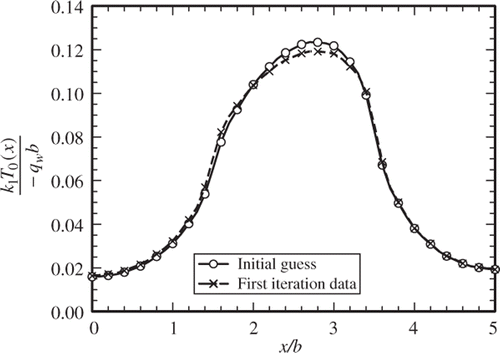
Figure 3. A comparison of computed values from first and second iterations.

Figure 4. A comparison of the computed values from third and fourth iterations.

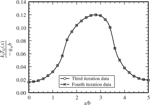
Figure 5. The deviations of from the previously determined values for each iteration.

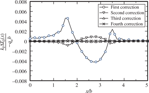
Table 1. Computed values of for the first four iterations.

	Initial	Diff.	1st	Diff.	2nd	Diff.	3rd	Diff.	4th
x/b
0.0	0.01586	0.0005	0.01637	−1E−04	0.01627	2E−05	0.01629	−4E−06	0.01629
0.2	0.01649	0.0007	0.01718	−1E−04	0.01707	2E−05	0.01709	−3E−06	0.01708
0.4	0.01803	0.0007	0.01870	−1E−04	0.01859	2E−05	0.01861	−4E−06	0.01861
0.6	0.02083	0.0007	0.02156	−1E−04	0.02143	3E−05	0.02146	−5E−06	0.02145
0.8	0.02522	0.0011	0.02631	−2E−04	0.02614	3E−05	0.02617	−5E−06	0.02616
1.0	0.03113	0.0012	0.03229	−2E−04	0.03208	4E−05	0.03212	−8E−06	0.03212
1.2	0.04022	0.0018	0.04202	−3E−04	0.04171	6E−05	0.04177	−1E−05	0.04176
1.4	0.05383	0.0031	0.05696	−5E−04	0.05649	8E−05	0.05657	−1E−05	0.05655
1.6	0.07764	0.0046	0.08223	−9E−04	0.08135	0.0002	0.08152	−4E−05	0.08149
1.8	0.09251	0.0018	0.09428	−4E−04	0.09389	9E−05	0.09398	−2E−05	0.09396
2.0	0.10401	−3E−04	0.10367	2E−05	0.10368	3E−06	0.10369	−2E−06	0.10369
2.2	0.11218	−0.002	0.11009	0.0004	0.11052	−9E−05	0.11043	2E−05	0.11045
2.4	0.11860	−0.003	0.11525	0.0007	0.11592	−1E−04	0.11578	3E−05	0.11581
2.6	0.12241	−0.004	0.11830	0.0008	0.11912	−2E−04	0.11895	4E−05	0.11899
2.8	0.12335	−0.004	0.11915	0.0009	0.12000	−2E−04	0.11982	4E−05	0.11986
3.0	0.12178	−0.004	0.11813	0.0007	0.11879	−1E−04	0.11866	3E−05	0.11869
3.2	0.11439	−0.002	0.11223	0.0004	0.11258	−6E−05	0.11252	1E−05	0.11253
3.4	0.09919	0.0015	0.10066	−4E−04	0.10023	0.0001	0.10034	−3E−05	0.10031
3.6	0.06713	0.0014	0.06851	−2E−04	0.06828	4E−05	0.06833	−9E−06	0.06832
3.8	0.04961	0.0004	0.05006	−1E−04	0.04994	3E−05	0.04997	−6E−06	0.04996
4.0	0.03803	0.0001	0.03816	−4E−05	0.03812	1E−05	0.03813	−3E−06	0.03813
4.2	0.03087	0.0003	0.03116	−6E−05	0.03110	1E−05	0.03111	−2E−06	0.03111
4.4	0.02538	5E−05	0.02543	−3E−05	0.02540	9E−06	0.02541	−2E−06	0.02541
4.6	0.02195	1E−04	0.02205	−2E−05	0.02202	6E−06	0.02203	−2E−06	0.02203
4.8	0.02015	0.0002	0.02030	−3E−05	0.02026	7E−06	0.02027	−1E−06	0.02027
5.0	0.01925	−6E−06	0.01925	−1E−05	0.01924	6E−06	0.01924	−2E−06	0.01924

The determination of temperature data at y = b, where the heaters are located, is important for the design and manufacturing of the devices where the temperature assumes its maximum values. Table 2 presents the computed temperature values at y = b for all four sets of iterations. The acquired data for these four iterations are plotted in Figure 6 and they indicate acceptable accuracies for practical applications. It is remarkable that the data for the first iteration are well behaved and they agree with subsequent iterations. Column 6 of Table 2 contains the numerically acquired data using ANSYS. This numerical model was developed so that it was not mesh sensitive. The data in column 6 agree reasonably well with those in column 7 of Table 2 that contains a set of computed temperatures using 500 eigenvalues followed by a sufficient number of iterations. The data in column 7 represent the exact values since they are accurate to all digits appearing in Table 2. These data show mixed agreements with those from the fourth iteration and the ANSYS data. The last column in Table 2 contains the percent deviation between the data in columns 5 and 6 of this table. Figure 7 shows the plotted temperature values for the fourth iteration and the ANSYS data, as presented in Table 2. This figure illustrates that 30 eigenvalues provide data that agree well with the numerically acquired information.

Figure 6. The temperature distribution over the heated surface as described by four successive iterations.

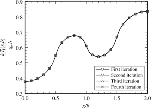
Figure 7. Temperature distribution over the heated surface after the fourth iteration for different Bi and the numerically computed data by ANSYS for Bi = 20.

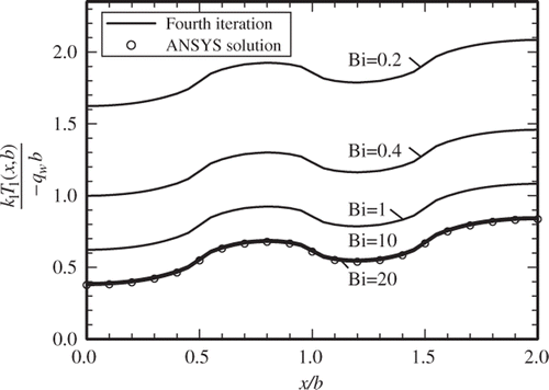
Table 2. Computed values of and their comparison with the numerically determined values by ANSYS.

							Percent
x/b	1st set	2nd set	3rd set	4th set	ANSYS	Exact	Difference
0.0	0.37734	0.37719	0.37721	0.37721	0.37715	0.37712	0.015
0.1	0.38183	0.38165	0.38167	0.38167	0.38170	0.38168	0.008
0.2	0.39575	0.39551	0.39555	0.39554	0.39583	0.39581	0.074
0.3	0.42113	0.42078	0.42083	0.42082	0.42141	0.42139	0.140
0.4	0.46353	0.46304	0.46312	0.46310	0.46350	0.46336	0.085
0.5	0.54857	0.54791	0.54803	0.54800	0.54893	0.54831	0.169
0.6	0.63165	0.63081	0.63096	0.63093	0.63093	0.63097	8E−04
0.7	0.66731	0.66629	0.66647	0.66644	0.66575	0.66567	0.104
0.8	0.67889	0.67770	0.67792	0.67787	0.67740	0.67733	0.069
0.9	0.66717	0.66581	0.66606	0.66601	0.66629	0.66633	0.041
1.0	0.60971	0.60821	0.60849	0.60843	0.60915	0.60853	0.117
1.1	0.55212	0.55051	0.55081	0.55075	0.55079	0.55063	0.007
1.2	0.54002	0.53833	0.53863	0.53858	0.53936	0.53932	0.146
1.3	0.55101	0.54927	0.54958	0.54952	0.55052	0.55049	0.183
1.4	0.58592	0.58414	0.58446	0.58440	0.58472	0.58457	0.055
1.5	0.66815	0.66636	0.66668	0.66662	0.66717	0.66653	0.083
1.6	0.75232	0.75054	0.75085	0.75079	0.75073	0.75076	0.008
1.7	0.79392	0.79217	0.79247	0.79241	0.79217	0.79208	0.031
1.8	0.81866	0.81692	0.81722	0.81716	0.81721	0.81713	0.006
1.9	0.83217	0.83044	0.83074	0.83068	0.83100	0.83092	0.039
2.0	0.83651	0.83479	0.83508	0.83503	0.83543	0.83535	0.048

4. Comments and discussions

This iterative procedure begins by properly selecting a function . This function is to be used in order to determine using Equation (19) and then obtain from Equations (11), (12a) and (12b). No iteration becomes necessary if the function obtained from Equation (14) is the same as the original heat flux function . The first iteration begins if these two quantities are different using the relation , as emerged from the solution of . The data acquired and presented in Table 1 show that, for a fixed number of terms in the series solution, only a few iterations are needed in order to get a relatively accurate solution. An alternative test shows that using a relaxation factor ω = 0.82–0.88 and selecting the new as (38) can improve the convergence rate.

The prepared computer program permits one to increase the number of iterations until a solution is obtained with a desired convergence for a fixed number of terms, N. Then, the temperature is computed with a high number of iterations using N = 30 terms. Selecting the data obtained from this solution as the reference values, the convergence due to the number of iterations was tested. With a relaxation factor of ω = 1, the data over y = b surface converged with deviations below after six iterations. However, with a relaxation factor of 0.85, only four iterations were needed in order to get alternative numerical results with deviations less than .

Minor modifications extend this procedure for the determination of temperature in three-dimensional bodies. Using the relation , the modifications begin by placing the eigenfunction in Equation (7) to get (39) wherein is the Kronicker delta while replaces the distance a and is the layer thickness in z-direction. Furthermore, the parameter can be obtained from the relation (40)

Next, the temperature solution in Layer 1 can be obtained by modifying Equation (13) to get (41)

Equations (24) and (25) would produce the temperature and heat flux relation over the surfaces at y = 0. Finally, the temperature solution in Layer 2 takes the form (42)

This leads to an iterative procedure similar to that discussed earlier.

5. Conclusion

The information presented earlier attests that the objectives of this study have been accomplished. It was demonstrated that only a few iterations were needed to achieve a satisfactory convergence and a faster convergence was realized with a properly selected relaxation factor. Furthermore, the convergence related to the number of eigenvalues was tested and it is a classical Fourier series issue.

This tested inverse procedure is equally applicable to three-dimensional cases as the inclusion of z-axis can be accommodated with ease, similar to that for the x-axis. Furthermore, this opens a path for future application of this iterative methodology to multi-layer bodies that are commonly used in electronic cooling applications. As an illustration, each of the two layers in Figure 1 is to be replaced by a block of layers with uniform footprints. The methodology for the determination of temperature in each block is given in 17.

References

- Goh, TJ, Thermal methodology for evaluating the performance of microelectronic devices with nonuniform power dissipation, 4th Electronics Packaging Technology Conference, Grand Copthorne, Singapore, 10–12 December, 2002, pp. 312–317.
- Sikka, KK, 2005. An analytical temperature prediction method for a chip power map. San Jose, CA: Semiconductor Thermal Measurement and Management Symposium, 21st Annual IEEE; 2005, pp. 161–166.
- June, MS, and Sikka, KK, Using cap-integral standoffs to reduce chip hot-spot temperatures in electronic packages, Thermal and Thermomechanical Phenomena in Electronic Systems, 8th ITherm Conference, San Diego, CA, 30 May–1 June, 2002, pp. 173–178.
- Zhiping, Y, Yergeau, D, Dutton, RW, Nakagawa, S, and Deeney, J, Fast placement-dependent full chip thermal simulation, VLSI Technology, Systems, and Applications, Hsinchu, Taiwan, 18–20 April, 2001, pp. 249–252.
- Mahajan, R, Nair, R, Wakharkar, V, Swan, J, Tang, J, and Vandentop, G, 2002. Emerging directions for packaging technologies, Intel Technol. J. Semiconduct. Technol. Manuf. 6 (2002), pp. 62–75.
- Kaisare, A, Agonafer, D, Haji-Sheikh, A, Chrysler, G, and Mahajan, R, 2009. Development of an analytical model to a temperature distribution of first level package with a non-uniformly powered die, J. Electron. Packag. 31 (2009), pp. 011005-1–011005-7.
- Beck, JV, Blackwell, B, and St. Clair, C, 1985. Inverse Heat Conduction: Ill-Posed Problems. New York: John Wiley; 1985.
- Alifanov, OM, and Nenarokomov, AV, 1999. Three-dimensional boundary inverse heat conduction problem for regular coordinate systems, Inverse Probl. Eng. 7 (1999), pp. 335–362.
- Alifanov, OM, and Nenarokomov, AV, 2001. Boundary inverse heat conduction problem: Algorithm and error analysis, Inverse Probl. Eng. 9 (2001), pp. 619–644.
- Silva, PMP, Orlande, HRB, Colaço, MJ, Shiakolas, PS, and Dulikravich, GS, 2007. Identification and design of source term in a two-region heat conduction problem, Inverse Probl. Sci. Eng. 15 (2007), pp. 661–677.
- Beck, JV, Blackwell, B, and Haji-Sheikh, A, 1996. Comparison of some inverse heat conduction methods using experimental data, Int. J. Heat Mass Tran. 39 (1996), pp. 3649–3657.
- Beck, JV, and Murio, DA, 1986. Combined function specification-regularization procedure for solution of inverse heat conduction problems, J. Am. Inst. Aeronaut. Astronaut. 24 (1986), pp. 180–185.
- Scheuing, JE, and Tortorelli, DA, 1996. Inverse heat conduction problem solutions via second-order design sensitivities and Newton's method, Inverse Probl. Eng. 2 (1996), pp. 227–262.
- Hào, DN, and Reinhardt, H-J, 1998. Gradient methods for inverse heat conduction problems, Inverse Probl. Eng. 6 (1998), pp. 177–211.
- Zhou, D, and Wei, T, 2008. The method of fundamental solutions for solving a Cauchy problem of Laplace's equation in a multi-connected domain, Inverse Probl. Sci. Eng. 16 (2008), pp. 389–411.
- Ling, X, Cheruturi, HP, and Keanini, RG, 2005. A modified sequential function specification finite element-based method for parabolic inverse heat conduction problems, Comput. Mech. 36 (2005), pp. 117–128.
- Haji-Sheikh, A, Beck, JV, and Agonafer, D, 2003. Steady state heat conduction in multi-layer bodies, Int. J. Heat Mass Tran. 46 (2003), pp. 2363–2379.