A note on the inverse mode shape problem for bars, beams, and plates

Abstract

Motivated by the idea of designing a structure for a desired mode shape, intended towards applications such as resonant sensors, actuators and vibration confinement, we present the inverse mode shape problem for bars, beams and plates in this work. The objective is to determine the cross-sectional profile of these structures, given a mode shape, boundary condition and the mass. The contribution of this article is twofold: (i) A numerical method to solve this problem when a valid mode shape is provided in the finite element framework for both linear and nonlinear versions of the problem. (ii) An analytical result to prove the uniqueness and existence of the solution in the case of bars. This article also highlights a very important question of the validity of a mode shape for any structure of given boundary conditions.

Keywords:

• inverse mode shape problem
• nonlinear eigenvalue problem
• valid mode shape

1. Introduction

A systematic methodology to design a structure to provide a particular mode shape is useful in many applications. For example, in capacitive resonant sensors, such as the coupled microcantilever gravimetric sensor 1, the deflections in resonant motion can be tailored to enhance sensing capability. Cantilever structures in the Atomic Force Microscopes point to another application where their probes can be designed for large tilts during their traversal at resonant frequency in the tapping mode 2. In vibration control, the amplitude of vibration at certain locations can be confined as desired by designing for mode shapes 3.

This article takes a step towards developing a numerical method to solve the inverse mode shape problem of finding the shape of regular structures such as bars, beams and plates. Although the ‘inverse frequency problem’ has been studied extensively 4,5, little work has been done on the ‘inverse mode shape problem’. These belong to a class of problems classified as partially described inverse eigenvalue problems 6.

This article is organized as follows. The next section deals with the work done earlier in the direction of solving the inverse eigenvalue problems involving bars, beams and plates. After this we present the inverse mode shape problem followed by the description of a numerical algorithm to solve the problem in the finite element (FE) framework. This is then followed by the results and discussion.

We then deal with the question of what exactly is a valid mode shape in the case of bars. It was first noted by Lai and Ananthasuresh 7 that any arbitrary function satisfying the boundary conditions need not be a valid mode shape and that they need to satisfy certain conditions. Similar conditions were identified for the fixed free boundary condition in bars by Ram and Elishakoff 8. This section generalizes these conditions for all boundary conditions, by analysing questions such as existence, uniqueness and construction procedure for a bar. Finally, conclusion and the challenges that lie ahead conclude this article.

2. Related work

The inverse eigenvalue problem was addressed by many authors. They aimed at determining both the geometric and material data of the structure. For bars, Ram and Gladwell 9 developed a procedure to find all the elements of the FE model matrices, i.e. the mass and stiffness matrices from two eigenvectors, one eigenvalue and total mass. This was further carried on, in the continuous case too, by Ram 10.

For the case of beams, Barcilon 11 developed a procedure for a beam clamped at one end and three spectra each with respect to three different boundary conditions at the other end to obtain a unique solution. Gladwell 12 established necessary and sufficient conditions for the reconstruction of the Euler–Bernoulli beam from spectral data.

In a generalized structure, a work by Burak and Ram 13 presented a numerical technique to solve the same problem under the knowledge of a single eigenvalue, two eigenvectors and a static deflection due to an unit load.

While the aforementioned works dealt with the problem of system identification, the inverse mode shape problem was introduced by Lai and Ananthasuresh 7 in the context of design. The problem they solved involved the knowledge of just one eigenmode and all parameters (mass, boundary conditions, Young's modulus, density) to determine the cross-section profiles of bars and beams. Ram and Elishakoff 8 elaborated upon this problem in the case of a fixed free bar where a discretized and analytical version of the problem was solved. Ananthasuresh 14 also extended these studies for the case of bars and beams with flexible supports. All the above-mentioned works have been based on finite difference discretization and have similar construction methodologies. They all concur that any possible admissible displacement cannot be a mode shape, and if it is a mode shape it can be used to determine the eigenvalue.

Our work rigorously justifies the preceeding statements for bars with any boundary condition in addition to presenting a solution algorithm in the FE framework for bars, beams and plates.

3. The inverse mode shape problem

Given the knowledge of material properties, boundary conditions, a constraint on the total mass and a desired mode shape, the objective is to find a suitable function for the design variables that governs the shape of the structure. This problem can be mathematically formulated for bars, beams and plates as described next.

3.1. Bars

The vibration of a bar of length L is governed by the differential equation, (1) where E, ρ, and A denote Young's modulus, density and the area of cross-section, respectively. All are positive quantities everywhere on the domain [0, L]. Symbol u refers to the modal displacement (i.e. the mode shape). λ is a positive constant, and is the square of the eigenvalue corresponding to the u(x). It may be noted that the equation for the inverse problem is linear in terms of A, which is the unknown function here.

3.2. Beams

The governing differential equation for the Euler–Bernoulli beam of length L is given by (2) where I stands for the moment of inertia of the beam, which is a positive quantity over the domain. The rest of the symbols carry the same meaning as in the case of bars. Contrary to the case of bars, here we have both I and A to be functions of the cross-sectional dimensions. As discussed in 7,14 a common parameterization for both can be found depending upon the shape and the cross-sectional dimension of interest. For example, if the beam is to be made with a rectangular cross-section, then we know that the moment of inertia is given by fracwidth × height³/12. If the height of the beam is fixed and the width is to be determined, then the problem is linear. On the other hand, if the width is fixed and the height is the unknown, then the problem becomes nonlinear. For convenience, we use the cross-section parameter c raised to power n to represent the moment of inertia of different cross-sections. Hence we have: (3)

3.3. Plates

As we extend the problem to plates, we need the thickness t(x, y) of the plate to be determined using the governing differential equation, (4) for Kirchoff Plates. The symbol ν is used to denote the Poisson's ratio, u(x, y) for the transverse displacement of the plate and the rest of the symbols have the same meaning as the previous cases.

In the discretized setting (e.g. FE, finite difference) all the three differential equations can be written as the generalized matrix eigenvalue problem: (5) where K(c) is the stiffness matrix and M(c) is the inertia mass matrix, both of which depend on the material properties and a set of cross-section parameters c.

In this work we develop a numerical technique to solve the problem in Equation (5) to find c for given u, material properties and boundary conditions. Also, one must note that the eigenvalue is unknown. From the numerical viewpoint, this problem poses a challenge as we are looking for the geometric parameter inside the matrix which occurs in a certain pattern inside the matrices K(c) and M(c).

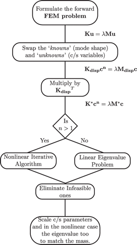
4. Numerical algorithm

The proposed algorithm is depicted in a flowchart in Figure 1. The central idea of this algorithm is ‘swapping’ variables u and c as originally proposed in 9 for a similar problem. We extend the same to formulate an eigenvalue problem. To understand this idea, let us consider a simple matrix equation expressed in two ways: (6) (7) It can be noticed that (6) and (7) are identical except that vector of variables [p, q, r]^T is swapped with [x, y, z]^T as the new variable vector in the matrix equation.

Figure 1. The numerical algorithm for solving the problem.

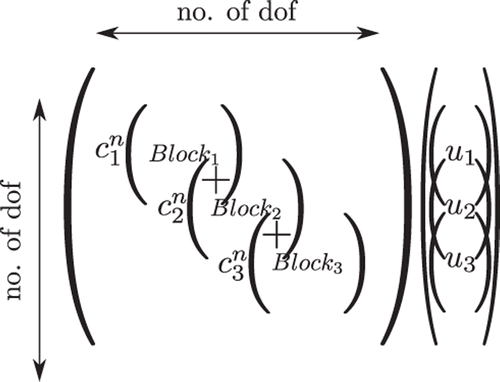
Be referring back to Equation (5), we note that, in the FE framework, matrices K and M are assembled as depicted in Figure 2. The assembly proceeds by the combination of the element matrices (indicated as Block_i) additively at their corresponding degrees of freedom (dof). If we assume the cross-section property to be a constant per element, then we can factor it out of the matrix as shown in Figure 2. For brevity, the entries corresponding to only three elements are shown in Figure 2.

Figure 2. The pictorial depiction of the assembly of the finite element matrices.

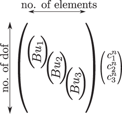
The square matrices K and M are of dimension equal to the dof after applying the boundary conditions. The geometric variables of interest are , and . The equation obtained after swapping is depicted in Figure 3. The element matrix without the unknown parameter is multiplied with the mode shape u corresponding to the element dof and assembled in the column corresponding to the element at the rows corresponding to the dof.

Figure 3. Here, Bu_i represents Block_i × u_i swapped form of the equation in Figure 2.

Let the matrix equations formed by this process be represented as (8) where the notation K_disp and M_disp denote the matrices formed after swapping the variables. So, they are functions of the modal displacements u while the cross-section parameters are taken outside and denoted by vector c. By the notation cⁿ we mean that each variable is raised to a power of n, as seen in Figure 3.

We reiterate that this recasting of the forward eigenvalue problem in terms of the displacements into the eigenvalue problem in terms of the cross-section parameters is the most crucial step in the numerical algorithm. This matrix system will be rectangular if the number of elements and the number of dof after applying boundary conditions are different. To avoid rank-deficiency, the system has to be just constrained (number of equations equal to the number of unknowns) or overconstrained (number of equations greater than the number of unknowns). This necessitates a proper choice of the interpolation for the displacement field to have an appropriate number of dof and nodes. For example, we had to use a three-noded element in the FE model for the bar instead of the more widely used two-noded one.

If an overconstrained rectangular system is obtained on swapping, i.e. K_disp and M_disp are rectangular, we pre-multiply it with its transpose analogous to the pseudo-inverse methodology to convert it to a square system as follows: (9) (10)

Now, the final equations become, (11)

If this problem is linear, i.e. n = 1, then it is a generalized eigenvalue problem with the feature that K* is symmetric and real, while M* is real but not symmetric. After the enumeration of the eigenvectors and eigenvalues, the unreasonable values such as, negative and complex eigenvalues, real eigenvectors with both positive and negative values are ignored. Finally, the reasonable possibilities have to be substituted back into the original rectangular equation (Equation (8) which is the one we have to solve) and the residual of the system is computed as (12) where | |₂ refers to the Euclidean norm.

If the residual is less than a tolerance value, the solution is acceptable. If we get no feasible solution or no solution with a sufficiently low residual, one may assume that the given mode shape might not have come out of such a governing differential equation, i.e., it is an invalid mode shape.

On obtaining an eigenvector, we know that it can be scaled by multiplying it with a scalar and it will still be a solution to the problem. To uniquely fix the eigenvector, the constraint of mass of the structure may be used to find this scaling factor. This is found by integrating a function of the cross-sectional dimensions, such as area × density, over the domain of the system as shown: (13)

Here, the scale factor is a constant that we have to find, Ω the domain and f the function of the cross-section parameter, which has to be integrated to get the mass. In all the cases considered the terms involving the scale factor can be factored out of integration as another function of it. Now, the integration is split across elements denoted by the subscript e and computed to obtain the scale factor.

For example, in the case of beams with a circular cross-section, if the radius is the geometric parameter (c), it translates to an integration of the form (14) We can factor out (scale factor)² and we can split the integration element by element as the cross-section parameter is a constant there. So, the integration of dx over the element gives the element length Length_e. Now, we get (15)

In the nonlinear case, when n ≠ 1 in Equation (11), an iterative approach similar in spirit to the power method 15 is used, as shown in a flowchart in Figure 4.

Figure 4. The flowchart illustrating the iterative technique for solving the nonlinear eigenvalue problem.

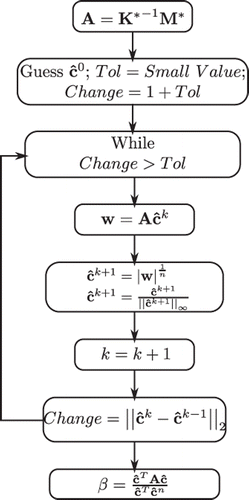
This algorithm can be understood if we re-write Equation (11) as (16) where (17)

Here, | |_∞ refers to the maximum norm.

This algorithm begins with a guess vector for that has all positive terms. When A multiplies , we get a vector w. If this were the solution, we would find it to be equal to . So, we find a, new by raising the absolute value (to maintain positive nature) of each term of w to the power and normalizing the resultant vector. We again multiply by A and repeat this procedure until convergence is achieved. After convergence we find β by, (18)

Now the residual of the original rectangular system, i.e. Equation (8) is computed as (19) If the residual is within tolerable limits, we can accept the converged result. We have noticed that the algorithm does not converge or the residual is not within tolerable limits if the mode shape is invalid, i.e. as explained before, a mode shape that is not a result of a governing differential equation for that structure.

When we have a solution, a scaling factor for is found by using the mass of the structure as described previously for the linear case. Additionally, here the eigenvalue changes as (20) In the next section, we present the results obtained by using this numerical technique.

5. Results and discussion

The numerical algorithm was tested with synthetic data. That is, first, a forward problem was solved with a particular set of cross-section parameters (also referred to as cross-section profile) and a mode shape was found. This was fed to the inverse problem and the results were compared against the inputs in the forward problem. The Young's Modulus used for all these cases is 210 GPa and the density is 7800 kg m⁻³ – the properties of steel.

5.1. Bars

The case of the bar is useful to understand the underconstrained (meaning fewer number of equations than unknowns) situation that occurs with the two-noded element. When the fixed-fixed end conditions are assumed for a two-noded element with one dof per node, the number of free dof (total number of elements −1) is just one short of the number of elements involved. The problem therefore becomes underconstrained. To avoid rank-deficiency, we took a three-noded element with constant element area which provides more equations than unknowns. Since it results in a linear eigenvalue problem, the solution was obtained using the ‘eig’ routine of Matlab (2007b, The MathWorks, Inc., Natick, MA, USA).

We demonstrate the algorithm with a few examples in Tables 1 and 2. The cross-section profile was plotted by assuming that the bar has a square cross-section. Also, by x we refer to the axial coordinate of the bar and by A we mean the area of the cross-section. Here and in forthcoming sections, by relative error in cross-section profile we mean, (21) where synthesized means the cross-sectional profile used in the forward problem and obtained means the result of the numerical technique used in the inverse problem.

Table 1. Examples for the inverse problem in bars: for each of these a 1 m long bar was discretized into 150 three-noded elements.

Table 2. Details for the examples in Table 1.

S. no	Boundary condition	Frequency (Hz)	Relative error in frequency	Relative error in cross-section profile	Residual
1	Fixed fixed	5.256 × 1E4	1E–14	1E–12	1E–10
2	Fixed free	5.682 × 1E4	1E–13	1E–12	1E–10

We notice that the relative errors are well within tolerance limits of E–10 or better. At this point, we would like to underscore that the algorithm yields only one unique solution when a valid mode shape (i.e. one obtained from the forward problem) is provided even though there is no restriction for other solutions to occur. In case an invalid mode shape is provided to the algorithm, it fails to yield any feasible solution as it either has an unacceptably high residual or fails to have a feasible solution. An invalid mode shape can be generated by randomly perturbing a valid mode shape by relatively small magnitudes.

5.2. Beams

We discretized the beams using the standard two-noded elements, with two dof per node. The Hermite interpolation for the element ensures that the problem is always overconstrained. As discussed in Section 3, the case of the beams can either be linear or nonlinear in terms of the cross-section parameter depending upon the parameterization.

Four examples, two for the linear and two for the nonlinear cases are illustrated in Tables 3 and 4. For the rectangular cross-section, when the height is constant, the equations are linear in terms of the width and it is nonlinear if we take the width to be constant and vary the height. For the circular cross-section, the problem is inherently nonlinear. The variables x and A have the same meaning as before. For the nonlinear inverse problem, the iterations were started with a uniform guess for the cross-section profile.

Table 3. Examples for the inverse problem in beams: for each of these a 1 m long beam was discretized into 100 two noded beam elements.

Table 4. Details for the examples in Table 3.

S. no	Boundary condition	Frequency (Hz)	Relative error in frequency	Relative error in cross-section profile	Residual
1	Fixed hinged	266.835	1E–12	1E–9	1E–10
2	Fixed free	311.035	1E–12	1E–9	1E–10
3	Fixed hinged	10725.280	1E–12	1E–12	1E–12
4	Fixed fixed	2039.164	1E–12	1E–10	1E–10

As seen in Table 4, the errors are well within tolerance and as in the previous case the linear case has only one feasible solution if the mode shape is valid. If it is invalid, then there is no feasible solution or the residual is far greater than the tolerance. In the nonlinear case we have noticed that it converges to the solution when the mode shape is valid and when it is invalid, either the residual is too high or else the iterations do not converge.

5.3. Plates

The cross-section profile has just one parameterization, namely the thickness. The equations are nonlinear in this. We used the Adini–Clough–Melosh, 4-noded elements, with three dof per node. This ensures that the problem is overcontrained. We illustrate two example in Tables 5 and 6. Here too, the iterations were begun with a uniform guess.

Table 5. Examples for the plate: for each of these a 1 m² plate was discretized into 30 × 30 four-noded plate elements.

Table 6. Details for example in Table 5.

S. no	Boundary condition	Frequency (Hz)	Relative error in frequency	Relative error in cross-section profile	Residual
1	Fixed on two opposite edges	2.470	1E–12	1E–10	1E–9
2	Fixed on all edges	1.347	1E–14	1E–13	1E–12

Table 6 shows that the results obtained are a good match for the synthetic data. But on varying the mode shape even very slightly, our algorithm either does not converge or yields unacceptably high residuals showing that the mode shape is invalid. From a practical standpoint, finding the structure with the closest possible mode shape to an invalid one is most important. This would use the traditional techniques of structural optimization, but the domain of functions to search for are governed by valid mode shapes. This led us to the investigation in the case of bars, where we prove the existence, uniqueness and conditions for a valid mode shape.

6. Valid mode shapes for a bar

We begin by defining what we mean by a ‘valid’ mode shape for a bar by referring to Equation (1) where u is the mode shape.

6.1. Valid mode shape

A valid mode shape is one that arises as a solution of Equation (1) which has the following properties built into it:

•	Area is strictly positive and C1 continuous.
•	Density is strictly positive and C0 continuous.
•	Young's Modulus is strictly positive and C1 continuous.
•	Boundary conditions such as the ones shown in Equation (22) are satisfied.

(22) The objective of this section is to propose and prove some lemmas to prove the following proposition.

Proposition 6.1

If the mode shape is valid, then the inverse problem of identifying the area and the eigenvalue from the mode shape, boundary conditions, mass constraint and material properties has a solution (existence) and it is unique (uniqueness).

Lemma 6.2

u and u′ cannot become zero simultaneously.

Proof

If u and u′ are simultaneously zero for a homogeneous linear second-order differential equation, by the theorem of uniqueness of ordinary differential equations 16 for initial value problems, there can only be a single possible solution and that is the null solution for u, which is not of interest to us. So u and u′ cannot be zero simultaneously. ▪

Lemma 6.3

The location where u′ vanishes fixes the eigenvalue, and the signs of u′′ and u′ are opposite at that point to ensure a positive eigenvalue.

Proof

Considering Equation (1) and substituting the condition that the derivative is zero and also noting that Lemma 6.2 implies that u is non-zero, we get the eigenvalue to be (23) As it is a valid mode shape, λ must be positive which indicates that u and u′′ must have opposite signs at that location to maintain positive sign.▪

Lemma 6.4

Wherever u′ vanishes, the eigenvalue prescribed by Equation (23) has to be the same.

Proof

As the mode shape is a valid one, the eigenvalue is unique for a mode.▪

Lemma 6.5

There exists at least one point in the domain where u′ becomes zero.

Proof

This is seen by the continuity of u and the boundary conditions. For the fixed-free and spring-free conditions, the derivative vanishes at the free end. Rolle's theorem guarantees the existence of at least one such point for the fixed-fixed condition.

The case where spring supports are present at both ends is handled as follows. Suppose we assume the contrary, i.e. u′ does not become zero anywhere in the domain. This implies that it should be of the same sign throughout the domain. Then, owing to the end conditions, , the above two statements imply that u must reverse sign.

Without any loss of generality, let u(0) be positive and so u′(0) has to be of the same sign too as both numerator and the denominator of have to be of the same sign to ensure positivity of the ratio.

Now u′(L) is also positive as the derivative is of the same sign throughout the domain.

The derivative being greater than zero implies that u should keep on increasing, i.e. it implies that u(L) > u(0), which is a contradiction to the deduction that u must reverse sign. So, u′ has to vanish at least at one point. An argument along similar lines yields the same conclusion even for the spring-fixed case.▪

Lemma 6.6

Both u and u′ possess isolated zeros (i.e. existence of at least a neighbourhood around a zero where the function does not vanish except at the location of the zero) 17.

Proof

If u is zero at a location, then u′ is not zero (by Lemma 6.2) and by the continuity of u′, one can find a neighbourhood where u′ is non-zero. This is the neighbourhood we are looking for, to prove the isolation of zeros of u. If u′ is zero then u is non-zero (by Lemma 6.2). If u is non-zero then by Equation (1) one can see that u′′ is non-zero. Now, again a similar argument proves the isolation of zeros of u′ too.▪

Lemma 6.7

The quantity – ((Eu′)′ + λρu′)/Eu′ has a limit at the point where u′ = 0 and is continuous in the rest of the domain.

Proof

If the mode shape is valid, the quantity under consideration is due to Equation (1) at locations where u′ is non-zero. However, is continuous everywhere in the domain. Taking the neighbourhood around u′ = 0 where it is non-zero (by Lemma 6.6) and the continuity of , we notice that the limit of the given quantity exists at that point.▪

Now, we are ready to prove Proposition 6.1 which aims at constructing a non-zero solution to the inverse problem.

Proof

λ can be found given a valid mode shape by Lemmas 6.3 and 6.4. It may be noted that, A is the unknown variable in Equation (1). Hence, we re-write the equation wherever u′ is not zero in a straightforward manner. When there is a singularity (i.e. u′ is zero), we take the limit of the term which is guaranteed to exist by Lemma 6.7. (24) The right-hand side of Equation (24) is a continuous function on the domain (by Lemma 6.7) and hence can be integrated over the domain to yield the solution. (25) The mass constraint fixes the arbitrary constraint C. Hence, this is a solution of the problem thereby guaranteeing the existence. Now for the uniqueness, suppose that there are two solutions to the above problem. Both will have to obey Equation (24), which means that both may differ only by a scale factor, which is determined by the mass constraint and provides us with the desired uniqueness if the mode shape is valid. Lemmas 6.3–6.5 guarantee uniqueness of the eigenvalue. This proves the proposition.▪

7. Conclusion and future work

This work presented a numerical solution methodology in the FE framework for the case of bars, beams and plates to solve the inverse mode shape problem. It also included an analytical study for the case of bars to prove the existence, uniqueness and construction procedure for the inverse mode shape problem. The numerical algorithm is suggestive of the uniqueness of the cross-sectional parameters in other cases too, but the proof is still open. On the numerical front, an algorithm that can give an estimate for cross-section properties that can generate the mode shape that is closest to the one required in case it is invalid, is also left for future work.

References

- Spletzer, M, Raman, A, Wu, AQ, and Xu, X, 2006. Ultrasensitive mass sensing using mode localization in coupled microcantilevers, Appl. Phys. Lett. 88 (2006), pp. 254102–254104.
- Pedersen, NL, 2000. Design of cantilever probes for atomic force microscopy (AFM), Eng. Optim. 32 (2000), pp. 373–392.
- Baccouch, M, Choura, S, El-Borgi, S, and Nayfeh, A, 2006. On the selection of physical and geometrical properties for the confinement of vibrations in non-homogeneous beams, ASCE J. Aerospace Eng. 19 (2006), pp. 158–168.
- Gladwell, GML, 2004. Inverse Problems in Vibrations, . Dordrecht: Kluwer Academic Publications; 2004.
- Chu, MT, 1992. Inverse eigenvalue problems, SIAM Rev. 40 (1992), pp. 1–39.
- Chu, MT, and Gene, HG, 2005. Inverse Eigenvalue Problems Theory, Algorithms, and Applications. Oxford: Oxford University Press; 2005.
- Lai, E, and Ananthasuresh, GK, 2002. On the design of bars and beams for desired mode shapes, J. Sound Vibration 254 (2002), pp. 393–406.
- Ram, YM, and Elishakoff, I, 2004. Reconstructing the cross-sectional area of an axially vibrating non-uniform rod from one of its mode shapes, Proc. Royal Soc. Lond. A 460 (2004), pp. 1583–1596.
- Ram, YM, and Gladwell, GML, 1994. Constructing a finite element model of a vibratory rod from eigendata, J. Sound Vibration 169 (1994), pp. 229–237.
- Ram, YM, 1994. An inverse mode problem for the continuous model of an axially vibrating rod, Am. Soc. Mech. Eng. Trans. J. Appl. Mech. 61 (1994), pp. 624–628.
- Barcilon, V, 1982. Inverse problems for the vibrating beam in the free-clamped configuration, Philos. Trans. R. Soc. Lond. A 304 (1982), pp. 211–252.
- Gladwell, GML, 1986. The inverse problem for the Euler–Bernoulli beam, Proc. R. Soc. Lond. A 407 (1986), pp. 199–218.
- Burak, S, and Ram, YM, 2001. The construction of physical parameters from modal data, Mech. Syst. Signal Proc. 15 (2001), pp. 3–10.
- Ananthasuresh, GK, 2004. "Inverse Mode Shape Problems for Bars and Beams with Flexible Supports". In: Inverse Problems, Design and Optimization Symposium. Rio de Janeiro, Brazil. 2004.
- Gene, HG, and Charles, FVL, 1996. Matrix Computations. Baltimore, MD: JHU Press; 1996.
- George, FS, 1991. Differential Equations with Applications and Historical Notes, . New York: McGraw-Hill; 1991.
- Al-Gwaiz, MA, 2008. Sturm Liouville Theory and its Applications. London: Springer-Verlag; 2008.