Abstract
The general method of iterative regularization is concerned with application to the estimation of material properties. The objective of this article is to estimate thermal and thermokinetic properties of advanced materials using the approach based on inverse methods. An experimental–computational system is presented for investigating the thermal and kinetics properties of composite materials by methods of inverse heat transfer problems and this is developed at the Thermal Laboratory of the Department of Space Systems Engineering, Moscow Aviation Institute. The system is aimed at investigating the materials in conditions of unsteady contact heating over a wide range of temperature changes and heating rates in vacuum, air and inert gas mediums.
1. Introduction
In spacecraft engineering, we deal with structures operating in the conditions of intensive, often extreme, thermal environments. For space re-entry vehicles and reusable transportation systems, the support of thermal conditions is one of the most important aspects of design, determining the main design solutions. Of great importance is the thermal merits support for different engines (gas turbine, liquid/solid propellant rocket engines, etc.), power plants, heat-exchange apparatus, etc. The distinctive features of modern heat-loaded structures in space engineering are non-stationarity, non-linearity, multidimensionality and conjugate nature of heat and mass transfer processes. These distinctions confine a possibility of using many traditional methods. So, in developing flight vehicles of different missions and types, traditionally there were both the development of new approaches and the improvement of available research techniques. Similar problems exist in other branches of industry.
Design optimization of heat-loaded objects as well as thermal control during operation time and corresponding emergency monitoring is actually an important problem in the presence of weight and cost restrictions on structures developed for any mission, for example, manned space stations, unmanned spacecraft and especially re-entry space systems like ‘Buran’, ‘Space Shuttle’, etc. The same problems are very important for internal combustion engines, nuclear power plants, metallurgical and chemical equipment, etc. A problem of reduction of specific consumption of materials of machines and vehicles, their power consumption and harmful action on the environment is extremely urgent in civil industries. Here, it is impossible to create heat protection systems, meeting modern requirements, without carrying out extensive theoretical and experimental studies of thermal state of the structures used Citation1–5. The priority and general orientation in the development of theoretical and experimental foundations of research, support and optimization of thermal conditions of structures of all prototypes of modern technology should be given to the development and broad application of methods of mathematical and physical simulation of a thermal state of the objects under study and, especially, experimental and computational methods of thermal diagnostics based on the solution of inverse heat and mass transfer problems. The research of recent years showed that the utilization of such an approach is most perspective and fruitful. It allows to take into consideration the actually existing effects of non-stationarity and non-linearity of heat and mass transfer processes; it displays high information efficiency and gives a possibility to conduct testing close to the maximum to full-scale or directly during operation of spacecraft Citation6–8.
The approaches to estimate thermal states of complex space structure based on methods of ill-posed problem solving were widely analysed in Russia and other countries, having displayed efficiency in the development and investigation of modern structure in rocket-space, aircraft, automotive industries, metallurgy, power engineering, etc. A new metrological system for thermal analysis of space structure being developed is a combination of sufficiently accurate measurements of primary heat values in testing conditions to the maximum approximate to full-scale conditions and ultimately correct mathematical treatment of experimental data based on the theory of inverse problems Citation9,Citation10.
In estimating temperature-dependent properties of modern composite destructive materials, the most effective are methods based on solution of the coefficient inverse heat transfer problems. The most promising direction in further development of research methods for destructive composite materials using the procedure of inverse problems is the simultaneous determination of a combination of material's thermal and kinetic properties (thermal conductivity , heat capacity
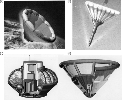
and some other parameters). Such problems are of great practical importance in the study of properties of composite materials used as destructive surface coating of spacecrafts Citation11,Citation12. The recently developed inflatable systems are based on destructive material coating ().
Figure 1. Inflatable structures: a, re-entry vehicle with inflatable aerodynamic shied; b, penetrator for Mars exploration; c, transportation; and d, inflatable structure installed.
The mathematical model of heat transfer in the specimen is
(1)
where the second term on the right-hand side covers the effect of convective heat transfer by the filtration of the gas that has arrived inside the material in the process of thermal kinetics (we make assumption that temperatures of the gas and the destructed material are equal), and the third term covers the specific heat of thermal kinetics.
(2)
(3)
(4)
(5)
(6)
(7)
(8)
In models (1)–(8), the coefficients ,
,
and
are unknown. The experimental equipment and the method described below could be applied for estimating the material's seven characteristics; the availability of a few specimens of the material allows us to provide uniqueness of the solution.
The results of temperature measurements inside the specimen are assigned as necessary additional information to solve an inverse problem
(9)
In the inverse problems (1)–(5), it is first of all necessary to indicate a temperature range of the unknown functions, which is general for all experiments and for which the inverse problem analysis has a unique solution. For
, the minimum value of initial temperature is used. Of much greater importance is a correct sampling of the
value. Proceeding from the necessity to provide uniqueness of solution, it seems possible to sample, for
, a minimum among maximum temperature values gained on the thermocouple positioned on the heated surface at every testing specimen.
2. Inverse problem algorithm
Suppose then that the unknown characteristics are given in their parametric form. With this purpose, introduce in the interval four uniform different grids with the number of nodes Ni, i = 1, … , 4.
(10)
The function
(11)
where
and
is called B-spline of the (j − 1) degree relatively with nodes
.
When solving practical problems, B-splines are used with so-called ‘natural’ boundary conditions
(12)
where u is the desired function.
Then, in case of cubic B-splines (j − 1 = 3), the unknown function is presented as
(13)
(14)
(15)
(16)
(17)
(18)
where
(19)
(20)
The function has the property
(21)
This property makes the computational algorithm simpler.
Approximating the unknown functions ,
,
and
on grids (11)–(21) using the cubic B-splines
(22)
(23)
(24)
(25)
where
, k = 1,N1,
, k = 1,N2,
, k = 1,N3,
, k = 1,N4 are the parameters.
As a result of approximation, the inverse problem is reduced to the search of a vector of unknown parameters ,
, with dimensions
. Writing down a mean-square error of the design and experimental temperature values in points of thermal sensors positioning
(26)
where
is determined from a solution of the boundary-value problems (1)–(8) using the approximations of (22)–(25). It is assumed here that the conditions of uniqueness of the inverse problem solving are satisfied.
A successive approximation method stated here, according to general definition of Tikhonov's regularizing operators, gives rise to a regularizing set of operators, in which a regularization variable is the number of the last iteration. For linear ill-posed problems, the iterative regularization method has received a rigorous mathematical substantiation and practical verification through data of mathematical modelling. There are at present no complete theoretical results on the substantiation of stability of iterative algorithms for non-linear problems. However, the results of computational experiments already made in solving the inverse heat transfer problems of different types prove the high efficiency of the iterative regularization method and possibility to analyse a wide range of non-linear problems.
So, proceeding from the principle of iterative regularization Citation1,Citation2, the unknown vector can be determined through minimization of functional (26) by gradient methods of the first order prior to a fulfilment of the condition
(27)
where
is the integral error of temperature measurements fm(τ), m = 1,M and
the measurement variance.
To construct an iterative algorithm of the inverse problem solving, a conjugate gradient method was used. The successive approximation process is constructed as follows:
| 1. | a priori, an initial approximation of the unknown parameter vector | ||||
| 2. | a value of the unknown vector at the next iteration is calculated | ||||
The greatest difficulties in realizing the gradient methods are connected with calculation of the minimized functional gradient. In the approach being developed, the methods of calculus of variations are used. Here, an analytic expression for the minimized functional gradient can be obtained
(29)
(30)
(31)
(32)
where
is the solution of a boundary-value problem adjoint to a linearized form of the initial problems (1)–(8).
(33)
(34)
(35)
(36)
(37)
(38)
(39)
(40)
To calculate the descent step, a linear estimation is used
(41)
using the boundary-value problem for the Freshet differential of T(x,τ) at the point {C(T),
,
, H(T)} (noted as
), and assumed to be given by
(42)
(43)
(44)
(45)
where
(46)
(47)
(48)
(49)
(50)
(51)
(52)
(53)
where
3. Experimental verification
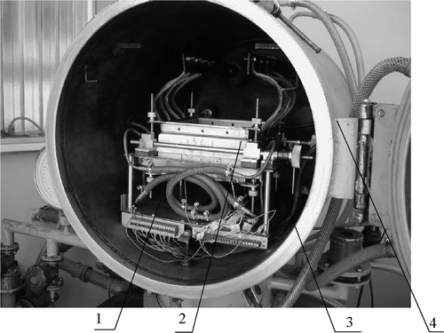
By the way of experimental study of the material specimens, the results of experiments are used on the automatic thermo-vacuum stand (TVS-1) manufactured in Moscow Aviation Institute at the Department of Space System Engineering. A TVS-1 is meant to carry out the experimental investigations on specimens of TPS materials in the condition of non-stationary radiation heating.
The test stand () consists of units and systems, described below. A horizontally set vacuum chamber 1 of 0.1 m3 volume is a cylinder with double walls between which the cooling water is circulating. A cylinder is sealed at both ends by spherical covers, the rear cover set fixed and the front cover hinged and provided with the quick-opening locks. Both covers are water-cooled too. A vacuuming system consists of a mechanic vacuum pump, a diffusion pump, a vacuum seal and valves. A power supply system includes a control desk, a thyristor voltage regulator, a control unit and a power transformer. A control unit is for voltage control fed to a heater. The control can be in a manual mode or automatic one from a computer.
Figure 2. Test stand: 1, vacuum chamber; 2, experimental module; 3, cooling system; and 4, electrical support.
Two specimens made of the same test material () were located symmetrically about the heating element on a thermoinsulating base made of thermal insulation material so that its heating surface is parallel to the heater and at a certain distance from it (δ = 4–5 mm). The other surfaces of specimens were heat-insulated by a layer of heat-insulating material. A heating element from a tantalum foil with dimensions 80 × 70 × 0.1 mm3 allowed: (1) to increase the specimen heating rate till the desired values and (2) to avoid destruction of heating elements till the completion of specimen tests, this having occurred sometimes in attempting to provide a corresponding heating rate. Control of the specimen heating condition is performed by temperature on the heated surface measured by a thermocouple made from a thermocouple wire BP5–BP20 of 0.1 mm diameter in accordance with a prescribed regime. A control system of the heating regime includes a thermocouple, set up on the specimen surface, a control-point setting device, operating jointly with a self-balancing electronic potentiometer and an analogy regulator device in the set with the control units. Control over the heating regime was maintained in the experiment by the results of three trial starts with specimens from test materials, the structure of which is similar to the structure used in tests. In making the trial starts, a criterion in choosing the suitable heating regime is the coincidence of the specimen external surface temperature measured with a prescribed temperature. Measurement and recording of non-steady temperatures in the test specimen are made by means of an automatic system for experimental information gathering and processing based on PC.
Figure 3. A testing scheme for specimens: 1, heating element; 2, thermoinsulated slab; 3, sensitive element (SE) of heat flux on the upper specimen; 4, upper specimen (1a/2a); 5, mask of the upper SE; 6, siding thermoinsulated slab; 7, voltage measuring point on the heater element; 8, lower specimen (B); 9, thermoinsulated slab; 10, SE on lower element specimen (B); 11, voltage measuring points on the heating element; 12, mask of the lower SE; and 13, siding thermoinsulated slab; T1, are the thermocouples on the heater; T2 − T6 the thermocouples on the upper specimen (A) and T7 − T11 the thermocouples on the lower specimen (B).
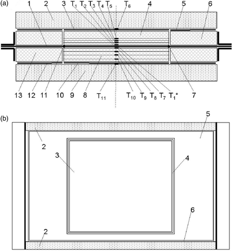
This module is implemented to provide a sufficiently exact definition of the heat flow fed inside the specimens of materials; this, in turn, permits to provide the conditions of uniqueness of the inverse problem solving by simultaneous definition of heat conduction and material's heat capacity per unit volume.
In the process of non-steady heating of specimens by means of an automatic system, recording of temperatures inside the specimen in place of thermocouple positioning, heater's temperature and also electric power released on it were performed
(54)
where U is the rms voltage on the heater and Ithe rms strength of current transmitted through the heating element. The heat flux supplied to a specimen due to symmetry is determined as
(55)
where A is the heater's surface area.
Comparisons of the calculated and measured temperatures on the specimen surfaces for testing material are presented in . The result of estimating the functions ,
,
and
for the material is presented in Figures . includes the obtained values of the least squares and the maximum deviation of the calculated temperatures from that measured in the experiments.
Figure 4. Comparison of the calculated (1–5) and measured (6–10) temperatures (specimen 1).
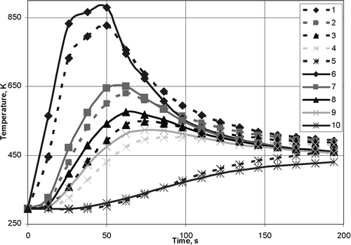
Figure 5. Estimated value of the heat capacity (specimens 1 and 2).
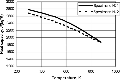
Figure 6. Estimated value of the thermal conductivity (specimens 1 and 2).
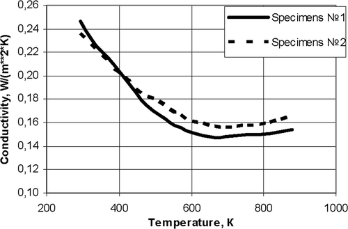
Figure 7. Estimated value of the gas heat capacity (specimens 1 and 2).
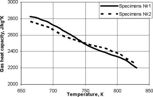
Figure 8. Estimated value of the heat effect (specimens 1 and 2).
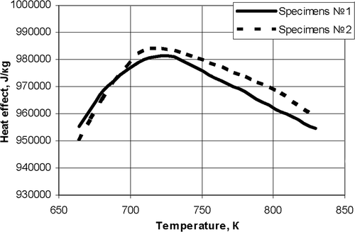
Table 1. The deviation of the calculated and measured temperatures.
4. Conclusions
This article seeks to describe the algorithm developed to process the data of unsteady-state thermal experiments. The algorithm is suggested for determining these unknown characteristics of a slab specimen as a solution of the non-linear inverse heat conduction problem in an extreme formulation.
The following main factors have an influence on the accuracy of the inverse heat conduction problem (in sequence of significance): the errors in coordinates of thermocouples’ positions; the errors in values of different characteristics; and the errors in estimating the residual level. For partially decomposed materials, the model of heat conduction with temperature-dependent thermal characteristics and one stage is approximate, and characteristics are effective, since the heat transfer in such a material is provided by heat conduction and a few different transformation processes depended on conditions of heating. A deviation of calculated and experimental temperature values in the experiments did not exceed 42 K that confirms the possibility of using, for the given material, a model of heat conduction with the effective thermokinetics. But this method can be used only for determining the effective thermal characteristics of composite materials for partial heating conditions.
Acknowledgement
This study was done with financial support provided by the Russian Government (grant no. NSh-65566.2010.8).
References
- Hansel, JG, and McAlevy, RF, 1966. Energetics and chemical kinetics of polystyrene surface degradation in inert and chemically reactive environments, AIAA J. 14 (1966), pp. 1055–1066.
- Lundell, JH, Dickey, RR, and Jones, JW, 1968. Performance of charring ablative materials in the diffusion-controlled surface combustion regime, AIAA J. 6 (1968), pp. 1115–1124.
- Pfal, RC, and Mitchel, BJ, 1970. Simultaneous measurement of six thermal properties of a charring ablator, Int. J. Heat Mass Transfer. 13 (1970), pp. 275–281.
- Potts, RL, 1990. Hybrid integral/quasi-steady solution of charring ablation. AIAA, Reston, VA: AIAA Paper No. 1677; 1990, 20p.
- Reinikka, EA, and Wells, PB, 1963. Charring ablators in lifting reentry. AIAA, Reston, VA: AIAA Paper No. 63–181; 1963, 15p.
- Vojvodich, NS, and Pope, RB, 1964. Effect of gas composition on the ablation behavior of a charring material, AIAA J. 12 (1964), pp. 536–542.
- Adarkar, DB, and Hartsook, LB, 1966. An integral approach to transient charring ablator problems, AIAA J. 14 (1966), pp. 2246–2248.
- Clark, BL, 1972. A parametric study of the transient ablation of teflon, Trans. ASME J. Heat Transfer. 94 (1972), pp. 347–354.
- Alifanov, OM, 1994. Inverse Heat Transfer Problems. Berlin/Heidelberg: Springer-Verlag; 1994.
- Alifanov, OM, Artyukhin, EA, and Rumyantsev, SV, 1995. Extreme Methods for Solving Ill-posed Problems with Applications to Inverse Problems. New York: Begell House; 1995.
- Artyukhin, EA, Ivanov, GA, and Nenarokomov, AV, 1993. Determination of a complex of materials thermophysical properties through data of nonstationary temperature measurements, High Temp. 31 (1993), pp. 199–202.
- Artyukhin, EA, and Nenarokomov, AV, 1987. Coefficient inverse heat conduction problem, J. Eng. Phys. 53 (1987), pp. 1085–1090.