Abstract
Traditional space-marching techniques for solving the inverse heat conduction problem are highly susceptible to both measurement and round-off error. This problem is exacerbated if the problem requires small time steps to resolve rapid changes in the surface condition, since this can cause instability. The inverse technique presented in this article utilizes a global time approach which eliminates the instability usually observed when using small time steps. It is demonstrated that a higher sampling rate (smaller time steps) in fact improves the inverse prediction. This is accomplished using a functional representation of the time derivative in the heat equation, and a physically based regularization scheme. A Gaussian low-pass filter is used with an analytically determined optimum cut-off frequency. The filter delivers an analytical function which has smooth, bounded derivatives. The inverse technique is demonstrated to accurately resolve the transient surface thermal condition in the presence of noise.
1. Introduction
The inverse heat conduction problem (IHCP) involves estimating the surface thermal condition without the use of surface-mounted sensors. Although the goal of the IHCP can be to resolve a variety of surface conditions – i.e. convection heat transfer coefficient, radiation heat transfer, surface heat flux and temperature – the projection techniques are generally identical. Resolution of the surface condition always involves projecting interior data (an ill-conditioned procedure) to the surface. IHCPs are of particular interest when the surface is under a harsh thermal environment, such as high temperatures and/or high heat fluxes, which precludes the use of sensors on the surface. Applications of the IHCP include atmospheric re-entry, solid rocket nozzles, hypersonic flow, quenching and fire research. A variety of methods have been employed to solve the inverse problem. These include ‘exact solutions’ Citation1, function specification Citation2–5, space marching and finite difference Citation6–12, non-integer system identification Citation13–15 and others Citation16–20.
The chief difficulty associated with the IHCP is that it is ill-posed, which complicates the resolution of the surface condition Citation21,Citation22. The physics of conduction provides a venue for the explanation of this phenomenon. In the forward (direct) problem, diffusion damps out high-frequency oscillation as the thermal front passes from the surface through the body. In the opposite direction (inverse), any high-frequency oscillations present in the data (i.e. noise) are amplified as the surface condition is projected from the sensor site Citation21,Citation22. Therefore, the inverse problem is highly sensitive to measurement error and must be ‘regularized.’
This study is motivated by the global time and global space paper of Frankel and Keyhani Citation23. In this article, we present a global time and discrete space formulation of the inverse problem. A novel treatment of the temporal derivative in the heat equation is utilized; namely, the time derivative in the heat equation is not finite differenced, and the in-depth data are projected directly to the surface without any need to compute the temperature at intermediate spatial nodes. A Gaussian low-pass filter is used for regularization. There are three main benefits to use this type of filter. First, this filter provides a global time regularization, i.e. all future and all past information is used in the regularization of the current time. Second, the output of this filter is an analytical function which can be analytically differentiated. Third, the filter ensures all time derivatives of the data to be smooth and bounded. The inverse technique presented in this article is demonstrated to be robust in the presence of noise. Additionally, refining the data sampling rate improves the inverse prediction rather than causing instability.
2. Problem description and inverse technique
Consider an isotropic, one-dimensional geometry with no internal generation and constant properties. The governing equation for this problem is given by the heat equation
(1)
where T = T(x,t) is the temperature, t is the time variable, x is the spatial variable, α is thermal diffusivity and L is the length of the (direct) spatial domain. Equation (1) is subject to an initial condition
(2)
for the entire spatial domain. The surface (x = 0) thermal condition is unknown
(3)
where k is the thermal conductivity. Heat flux and temperature data are provided at the embedded sensor site (x = d) such that
(4)
(5)
where q0(t) is the heat flux data and T0(t) is the temperature data.
The goal of the inverse problem is to resolve the unknown surface (x = 0) thermal condition using the provided sensor (x = d) temperature and heat flux data. This can be accomplished by first discretizing space such that xj = (N − j)Δx, i.e. xj=0 corresponds to the sensor site (x = d) and xj=N corresponds to the surface (x = 0). The spatial derivative of the heat equation in Equation (1) is approximated using a central difference as
(6)
Traditionally, the time derivative is also approximated using a difference formula. However, if the heating rate and higher time derivatives of temperature are directly measured Citation24 or can be obtained via post-processing, then time need not be differenced. We, therefore, define the operator, F, as
(7)
and solve Equation (6) for Tj + 1 to obtain
(8)
An energy balance at the sensor site (j = 0) yields the result
(9)
where T0(t) and q0(t) are the sensor data. Using a process of repeated analytical substitution with Equations (8) and (9), the temperature at the Nth spatial node (i.e. at the surface) can be solved in terms of the sensor temperature and heat flux explicitly. As an example, for N = 4 and N = 7 the equations are
(10)
(11)
respectively. For resolution of the surface temperature, N temporal derivatives of temperature data and N − 1 temporal derivatives of the heat flux data are required. An energy balance at the surface yields
(12)
which again can be found explicitly in terms of sensor temperature and heat flux only. As an example, Equation (12) for N = 4 and N = 7 becomes
(13)
(14)
For resolution of the surface heat flux, N + 1 temporal derivatives of the temperature data and N temporal derivatives of the heat flux data are required. Therefore, if noise exists in the sensor data, the projection process is clearly ill-posed. Additionally, if the derivatives are obtained numerically, significant round-off error will accumulate as N increases, and again the process is ill-posed. However, if the data and the required number of temporal derivatives are bounded and smooth, the projection process is well-posed. This can be accomplished via a low-pass Gaussian filter.
3. Regularization via digital filtering
As discussed above, high-frequency oscillations present in the data (noise) cause the inverse projection to become unstable. The reason for this is made clear through inspection of Equation (13). For N = 4, five time derivatives of the temperature data and four time derivatives of the heat flux data are required to resolve the surface heat flux. Time-differentiating noisy data produces an unbounded and unstable result. A physically meaningful way of stabilizing the inverse problem is to remove the non-physical, high-frequency energies from the signal by way of a low-pass digital filter. Consider the Gaussian low-pass filter given by
(15)
where fc is the cut-off frequency in hertz,
is the filtered temperature and
denotes the raw, discrete sensor data. Derivatives of Equation (15) can be obtained analytically; the first time derivative is given by
(16)
The output of Equations (15) and (16) are analytical functions which remove high-frequency energies (noise) from the signal and ensure continuous, smooth temporal derivatives Citation22 as required by the inverse technique. Therefore, a carefully chosen cut-off frequency is the only parameter necessary to regularize the data and make the problem well-posed.
The cut-off frequency of the filter can be determined using residual minimization in the least-squares sense. Traditional least squares would seek to minimize the difference between the filtered and noisy data, i.e. the residual. However, some authors Citation25,Citation26 have noted that the difference between the filtered and the exact data should be minimized. First, let us define the noisy data to be
(17)
where ε is the noise which is considered to be of a Gaussian distribution with a constant standard deviation, σ, and has a zero mean. Next, we define the residual as the difference between noisy and filtered data such that
(18)
Clearly, minimizing the difference between the filtered and exact data is the same principle as setting the residual equal to the noise. Therefore, we utilize the Euclidean norm and seek to minimize the function
(19)
where ton is the time at which the source at the surface is switched on and tmax is the time at the final data sample. The discrete 2-norm is defined here as
(20)
The function, φ1, now contains the noisy data, filtered data and the noise history. Additionally, lead data is commonly taken before the source is turned on. We use the mean of the lead data, Ti (initial condition), to define φ2 as
(21)
where Ti is again the initial condition. The cut-off frequencies which produce minimums of φ1 and φ2 provide a range of optimal cut-off frequencies from which the user can choose. It should be noted that the Gaussian low-pass filter of Equation (15) is not overly sensitive to the choice of cut-off frequency; a change of 15–20% will not dramatically influence the filtered data.
At first, this procedure does not seem useful since in the real world both the exact data and the noise history are unavailable (apart from the initial condition). However, we utilize a procedure of estimating the noise outlined in Frankel et al. Citation25. A first-order polynomial is fit to the noisy data, and the residual, R1(tk), between the noisy data and the first-order least-squares fit is calculated. Next, a higher order function, , is used to approximate R1(tk) via least squares. The error is then estimated as
(22)
4. Errorless data
For demonstration, consider a pulsed surface heat flux given by
(23)
where qS is the peak source heat flux, H is the Heaviside step function Citation27 and tm are the time values for switching the surface flux on and off. For this article, we wish to observe lead data (before surface heat flux is turned on), one pulse and cooling data. Therefore, tm=0 = ton and tm=1 = toff. Without loss of generality, we use the half-space as the domain, noting that this is valid until the thermal front reaches the back wall (x = L).
The exact solution for the forward problem is given by Frankel et al. Citation28
(24)
and
(25)
Without loss of generality, the results we present are made dimensionless via
(26)
(27)
(28)
(29)
(30)
where Fo is the dimensionless time, η is the dimensionless space, θ is the dimensionless temperature,
is the dimensionless heat flux and
is the dimensionless frequency. Note that although the peak source heat flux, qS, is unknown a priori, it is merely a scaling factor in Equations (28) and (29). Therefore, the actual value of qS is unimportant for this analysis.
Although the exact solution for this problem is available, the digital filter was used to show its performance. The exact solution for temperature and heat flux Equations (24) and (25) were ‘sampled’ at a given rate, and the data were provided to the Gaussian low-pass filter. Since errorless data were used (i.e. no regularization needed), a suitably high dimensionless cut-off frequency of
was used in the filter for both temperature and heat flux data. The output of the filter was then provided as input to the projection scheme.
Inverse temperature and heat flux results for N = 4 can be seen in using a sampling rate of The inverse method does an excellent job of capturing the jump in heat flux at Fo = 0.5, with only a short lag. The accuracy of the inverse method should improve as the order of the projection (N) increases. shows the inverse heat flux results for N = 7 with all other parameters unchanged. Although increasing the projection order should have had a positive effect on the results, a bias in the heat flux prediction is observed. This is because the dimensionless sampling rate of
for N = 7 is slow; as the projection order increases, the data density required to resolve the higher order temporal derivatives via the filter also increases. shows the inverse heat flux results for N = 7, but with an increased sampling rate of
As the sampling rate is increased, the results are still stable, and the bias in the heat flux prediction vanishes.
Figure 1. Inverse results using N = 4 using errorless data: (a) temperature and (b) heat flux inverse predictions.
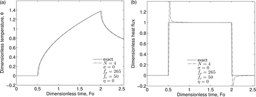
Figure 2. Effect of the sampling rate on the inverse heat flux prediction with N = 7 using errorless data: (a) and (b)
.
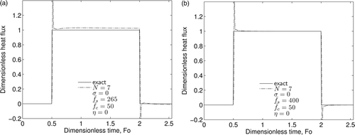
If the sampling rate is appropriately fast, use of more spatial nodes will also enable the inverse method to capture a change in the surface condition more quickly. and illustrate this quite well. For N = 7, the response time when both the sources are turned on and off is much faster than for N = 4. Additionally, the Gibbs’ spike is also seen to decrease with increasing N. These observations make physical sense for two reasons. First, as N increases, space becomes less lumped and more continuous, i.e. more accurate. Second, increasing N increases the highest order of time derivative used in the inverse prediction. Each higher time, the derivative picks upon changes in boundary conditions faster than the previous derivative, which will result in a faster response time. In sharp contrast to other inverse methods, this implies that one should use the largest N possible with the highest sampling rate available.
5. Noisy data
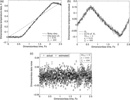
For demonstration, again we consider a pulsed surface heat flux given by Equation (23) with the exact solution given by Equations (24) and (25). Noise is simulated using dimensionless variables and a random Gaussian distribution with a constant dimensionless standard deviation of 0.01 and a zero mean. This noise is added to the temperature and heat flux data as in Equation (17). The cut-off frequency for the low-pass Gaussian filter must then be found. This is accomplished by first obtaining an estimate for the noise history as outlined in Frankel et al. Citation25. A first-order polynomial is fit to the noisy data, and the residual, R1, between the noisy data and the first-order least-squares fit is calculated. Next, a higher order function is used to approximate R1, and the residual between this fit and R1 is used as the estimated noise history. shows the noisy data and a one-term least-squares fit of the data. shows the residual, R1, and an eighth-order least-squares fit of R1. Here, the function used to fit the residual is of the form
(31)
where Ωm(t) are the basis functions and am are the unknown coefficients. We have used the Hardy multiquadric radial basis functions given by
(32)
where tm and βm are the mth centre and shape factor, respectively. As in Citation25, we have used equidistant centres tm = mtmax/M and set βm = β = (tmax/M)2. The recreated noise and the actual noise can be seen in . Clearly, this is an effective tool for estimating the noise present in the data.
Figure 3. Technique for estimating the noise present in the data: (a) first-order fit to data; (b) least-squares fit to residual; and (c) actual and estimated noises.
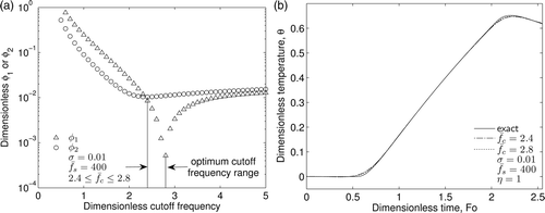
Once the noise history has been estimated, φ1 and φ2 from Equations (19) and (21) can be used to provide a range of appropriate cut-off frequencies. This can be seen in where the reported optimum dimensionless cut-off frequency range is 2.4–2.8. As noted above, the Gaussian low-pass filter used here is relatively insensitive to the actual choice of cut-off frequency. shows the noisy and filtered temperature histories using cut-off frequencies of 2.4 and 2.8. Although there is a 17% difference between these two values of cut-off frequency, the filter outputs are nearly graphically identical.
Figure 4. Gaussian low-pass filter exploration: (a) optimum cut-off frequency range and (b) insensitivity of Gaussian filter to a small change in cut-off frequency.
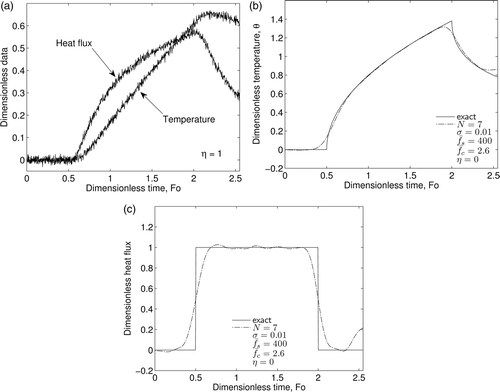
shows the effectiveness of the inverse method in the presence of noise. Noise was simulated using a normal distribution with a standard deviation of 0.01 for both dimensionless temperature and heat flux data and can be seen in using a sampling rate of Optimum cut-off frequency ranges were determined to be 2.4–2.8 for the temperature data and 1.7–3.9 for the heat flux data. For simplicity, a common cut-off frequency of 2.6 was used for both temperature and heat flux data. The data were filtered and passed to the inverse scheme. The resulting inverse predictions of the surface temperature and heat flux histories can be seen in , respectively. A smoothing effect is observed near ton and toff. Once the inverse prediction settles, the standard deviation of the error is calculated to be 0.01 in the domain 0.75 ≤ Fo ≤ 1.75, which is exactly the same as input error. Additionally, further refinement of the sampling rate does not adversely affect the inverse results. The regularization and inverse method combination effectively makes the problem well posed.
Figure 5. Inverse results using a normal distribution, with a standard deviation of 0.01 and a dimensionless cut-off frequency of 2.6: (a) noisy data used as input to the inverse code; (b) inverse temperature results and (c) inverse heat flux results.
In order to demonstrate the generality of this inverse technique, we also present the classical Beck triangle problem Citation21. The surface boundary condition is defined as
(33)
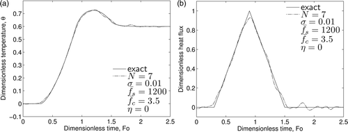
The body is insulated at x = L, and the sensor is located at x = d = L. For a dimensionless sampling rate of noise is simulated as in Equation (17) using a normal distribution with a zero mean and a standard deviation of 0.01 for dimensionless temperature which can be seen in . The optimum cut-off frequency range for the data presented was determined to be 2.1–4.9. As noted above, the Gaussian low-pass filter used here is relatively insensitive to the actual choice of cut-off frequency. shows the exact and filtered temperature histories using cut-off frequencies of 2.1 and 4.9. Although there is a large difference between these two values of cut-off frequency, both filter outputs approximate the temperature data well. As a compromise between these two values, a dimensionless cut-off frequency of 3.5 was used to filter the data. The filter output was then passed to the inverse code; the results for the predicted surface temperature and heat flux histories can be seen in . The peak value of heat flux is underestimated by only 7.0%.
Figure 6. Temperature data for Beck triangle problem: (a) raw data with σ = 0.01 and (b) insensitivity of Gaussian filter to change in cut-off frequency.
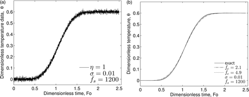
Figure 7. Inverse results for the classical Beck triangle problem for: (a) surface temperature prediction and (b) surface heat flux prediction. Noise was simulated using a normal distribution, σ = 0.01 and used for regularization.
An investigation of the accuracy of the proposed inverse method as a function of the sampling rate was conducted using the surface heat flux of Equation (33) as the test case. The sampling rate was varied from 100 ≤ ≤ 1200. Five unique random error distributions were generated for each sampling rate and added to the data as in Equation (17). The RMS of the surface inverse heat flux prediction was calculated for each dataset such that
(34)
where M is the number of time samples. The RMS error was averaged for the five runs at each sampling rate. Two different values for the order of the inverse scheme, N = 4 and N = 7, were used. The cut-off frequency was chosen as the midpoint of the optimum range from φ1 and φ2 for both values of N. Also, for N = 7,
was held constant at
to investigate the effect of sampling rate independent of the cut-off frequency.
presents the results of the accuracy investigation. In sharp contrast to other inverse methods Citation21, for N = 4 or N = 7, increasing the sampling rate resulted in a decrease of the error norm. This is because the time derivatives of the temperature data are more accurately resolved at higher sampling rates. These results hold whether the cut-off frequency is kept constant at 3.0, or chosen as the midpoint of the optimum range. Additionally, greater accuracy was achieved using the proposed analytical method of determining cut-off frequency over holding the cut-off frequency constant at Next, it was observed that the error norm improved as N was increased (i.e. more spatial nodes) from N = 4 to N = 7 using the proposed cut-off frequency determination method. Minimal improvement occurred for low sampling rates, while greater improvement occurred as the sampling rate was increased. Again, this is because the higher time derivatives of the temperature data are more accurately resolved at higher sampling rates; hence, greater improvement is seen at higher sampling rates. These results suggest that optimum inverse predictions are obtained by sampling the data at the highest possible rate, using higher number of spatial nodes (N), with the proposed cut-off frequency determination method.
Table 1. Predicted heat flux RMS error as a function of the sampling rate,  , projection order, N and choice of cut-off frequency,
  and qRMS,mean are average values resulting from five independent noise distributions.
6. Conclusions
A robust global time inverse heat conduction method has been demonstrated. In stark contrast to traditional inverse methods, increasing the data density does not compromise stability of the inverse prediction. Indeed, the inverse results improve with faster data sampling. The time derivative of the heat equation is not finite differenced. Instead, a functional representation of the higher time derivatives of temperature are used to project directly to the surface without the need to calculate the temperatures at intermediate spatial nodes. This is accomplished via a low-pass Gaussian filter with a physically based cut-off frequency which provides an analytical function as output. The proposed regularization scheme presented provides bounded, continuous, analytical time derivatives of the sensor data. Additionally, an analytical method for determining the optimum filter cut-off frequency range is demonstrated. The novel treatment of the temporal derivative in the heat equation, combined with the global time Gaussian low-pass filter, provides the regularization required for stable, accurate results. Future studies with this concept should involve extension to two- and three-dimensional geometries.
Acknowledgements
The results presented in this article were partially supported under the NASA Cooperative Agreement NNX10AN35A.
References
- Burggraf, OR, 1964. An exact solution of the inverse problem in heat conduction theory and application, J. Heat Transfer 86 (1964), pp. 373–382.
- Beck, JV, , Calculation of surface heat flux from an internal temperature history, ASME Paper no. 62-HT-46, 1962.
- Kurpisz, K, and Nowak, AJ, 1995. Inverse Thermal Problems. Southampton: Computational Mechanics Publications; 1995.
- Beck, JV, Blackwell, B, and Haji-Sheikh, A, 1996. Comparison of some inverse heat conduction methods using experimental data, Int. J. Heat Mass Transfer 39 (17) (1996), pp. 3649–3657.
- Beck, JV, 2008. Filter solutions for the nonlinear inverse heat conduction problem, Inverse Prob. Sci. Eng. 16 (1) (2008), pp. 3–20.
- D'souza, N, , Numerical solution of one-dimensional inverse transient heat conduction by finite difference method, Winter Annual Meeting, ASME Paper no. 75-WA/HT-81, Houston, TX, 1974.
- Elkins, BS, Keyhani, M, and Frankel, JI, , Methodology for stable and accurate resolution of the inverse heat conduction problem, Int. J. Numer. Methods Eng., in review.
- Carasso, AS, 1992. Space marching difference schemes in the nonlinear inverse heat conduction problem, Inverse Prob. 8 (1) (1992), pp. 25–43.
- Carasso, AS, 1993. Slowly divergent space marching schemes in the inverse heat conduction problem, Numer. Heat Transfer, Part B 23 (1) (1993), pp. 111–126.
- Al-Khalidy, N, 1999. Analysis of boundary inverse heat conduction problems using space marching with Savitzky-Gollay digital filter, Int. Commun. Heat Mass Transfer 26 (2) (1999), pp. 199–208.
- Murio, DA, and Hinestroza, D, 1993. The space marching solution of the inverse heat conduction problem and the identification of the initial temperature distribution, Comput. Math. Appl. 25 (4) (1993), pp. 55–63.
- Taler, J, 1999. A new space marching method for solving inverse heat conduction problems, Forschung im Ingenieurwesen 64 (11) (1999), pp. 296–306.
- Lohle, S, Battaglia, JL, Batsale, JC, Bourserau, F, Conte, D, Jullien, P, Ootegem, B van, Couzi, J, and Lasserre, JP, , Estimation of high heat flux in supersonic plasma flows, Proceedings of IEEE Industrial Electronics, IECON, Paris, 2006.
- Lohle, S, Battaglia, JL, Batsale, JC, Enouf, O, Dubard, J, and Filtz, JR, 2007. Characterization of a heat flux sensor using short pulse laser calibration, Rev. Sci. Instrum. 78 (5) (2007), p. 6.
- Battaglia, JL, Cois, O, Puigsegur, L, and Oustaloup, A, 2001. Solving an inverse heat conduction problem using a non-integer identified model, Int. J. Heat Mass Transfer 44 (14) (2001), pp. 2671–2680.
- Taler, J, 1996. A semi-numerical method for solving inverse heat conduction problems, Heat Mass Transfer 31 (3) (1996), pp. 105–111.
- Kim, SK, and Lee, WI, 2002. Solution of inverse heat conduction problems using maximum entropy method, Int. J. Heat Mass Transfer 45 (2) (2002), pp. 381–391.
- Özisik, MN, and Orlande, HRB, 2000. Inverse Heat Transfer. New York: Taylor & Francis; 2000.
- Shen, SY, 1999. A numerical study of inverse heat conduction problems, Comput. Math. Appl. 38 (7–8) (1999), pp. 173–188.
- Deng, S, and Hwang, Y, 2006. Applying neural networks to the solution of forward and inverse heat conduction problems, Int. J. Heat Mass Transfer 49 (25–26) (2006), pp. 4732–4750.
- Beck, JV, Blackwell, B, and St Clair, CR, 1985. Inverse Heat Conduction. New York: Wiley; 1985.
- Frankel, J, 2007. Regularization of inverse heat conduction by combination of rate sensor analysis and analytic continuation, J. Eng. Math. 57 (2) (2007), pp. 181–198.
- Frankel, JI, and Keyhani, M, 1997. A global time treatment for inverse heat conduction problems, J. Heat Transfer 119 (4) (1997), pp. 673–683.
- Elkins, BS, Huang, M, and Frankel, JI, 2012. In-situ higher-time derivative of temperature sensors for heat transfer, Int. J. Therm. Sci. 52 (2012), pp. 31–39.
- Frankel, JI, Keyhani, M, and Taira, K, 2004. In-phase error estimation of experimental data and optimal first derivatives, AIAA Journal 42 (5) (2004), pp. 1017–1024.
- Murio, D, 2002. Mollification and Space Marching. Boca Raton, FL: Inverse Engineering Handbook, CRC Press; 2002.
- Abramowitz, M, and Stegun, IA, 1965. Handbook of Mathematical Functions. New York: Dover; 1965.
- Frankel, JI, Osborne, G, and Taira, K, 2006. Stabilization of ill-posed problems through thermal rate sensors, J. Thermophys. Heat Transfer 20 (2) (2006), pp. 238–246.