Practical considerations when using sparse grids with Bayesian inference for parameter estimation

Abstract

When estimating parameters it is important to determine both the most probable values and the confidence intervals. To do so accurately requires Bayesian inference that can involve a high computational cost for complex models, particularly if the range of possible parameter values is large. One approach is to sample the model response surface and to interpolate. When done with a tensor grid the cost of developing an accurate representation of the surface and to locate the point of greatest probability can be prohibitively expensive. Sparse grids offer an alternative that may be of less cost. Because sparse grids are inherently approximations it is important to determine the accuracy of the representations since the errors may lead to less efficient calculations in estimating parameters and may distort the marginal probability distributions of the parameters. Except for atrociously ill-conditioned inverse problems sparse grids are particularly well suited for use with the least-squares approach and are even better for Bayesian inference and the detection of the cause of ill-conditioning.

Keywords:

• sparse grids
• hierarchical Bayesian inference
• parameter estimation

1. Introduction

The standard approach to estimating parameters is the least-squares analysis in which the estimated parameters are those that minimize the norm of the residuals based upon the fundamental assumptions that the model is correct and that any deviation of the data from the model is due to normally distributed zero mean errors. An important aspect of the inverse problem is the estimation of the standard deviation of the estimated parameters. In the least-squares approach we define the model as M(Θ), where Θ represent the set of parameters. Let the true value of the parameters be denoted by Θ and the estimated values by . The measurements, D, are presumed to be corrupted by the noise ε to give (1) where E[ε] = 0 and cov[ε] = Σ. For non-linear problems, the parameters are found using a solution that is effected by an iterative procedure based upon linearization. The estimated property, , is that which minimizes the functional (2) where the residuals r are defined by (3) Linearizing Equation (2b) about an estimate Θ_i gives (4) and is given by (5) where . For N measurements and d parameters, D and M are [N × 1] vectors, Θ is a [d × 1] column vector, A is a [N × d] matrix and β, the Levenberg–Marquardt (LM) parameter 1, is used for ill-conditioned problems. Upon convergence of the iterations, the estimate satisfies (6) (7)

Equations (3b) and (3c) represent the generally acceptable desirable state of being an unbiased estimator with minimum variance 2. To determine one must know the covariance matrix Σ of the noise. Σ can be expressed in terms of the correlation matrix Ω as (8) Ω can usually be obtained by standard statistical analyses 3 taking into account any autocorrelation. If Σ is not known, one usually investigates the statistics of the residuals, which if Σ = σ_nI satisfy (9) (10) where σ_n is the standard deviation of the noise. Unfortunately this estimate of often seriously underestimates the range of probable values especially when is not normally distributed.

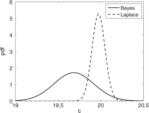
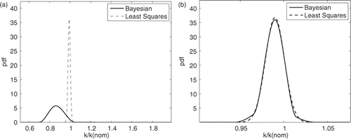
A better approach is based upon hierarchical Bayesian inference 4,5 that allows us to incorporate knowledge about the reasonable values of the parameters sought and information about any other parameters involved in the model. Figure 1 compares the probability distribution (pdf) for the specific heat, c, obtained from least-squares based on Laplace's assumption (namely that the distribution is assumed to be normally distributed about with the standard deviation given by Equation (3c)) with the marginal distribution obtained from Bayesian inference when estimating the specific heat from the transient conduction problem described later in this article. Note that the breadth of the distribution based upon the Bayesian approach is substantially greater and that an estimate of the uncertainty of based upon least-squares is a significant under estimate.

Figure 1. Comparison of the pdf () for Problem 1.

Unfortunately for many real problems, the computational expense for Bayesian inference is prohibitively high. One solution is to use an interpolation of the response function, but this is usually only realistically possible if the interpolation is cheap. Sparse grids offer a possible approach, but they have problems of their own. This article describes the use of sparse grids and offers some practical advice for their effective use in Bayesian inference.

2. Bayesian inference

The Bayesian approach consists of determining the marginal distribution of a single parameter under the assumptions for prior knowledge of the parameters and of any other unknown elements. Consider the case of two parameters to be estimated, Θ₁, Θ₂, from a set of data D that is presumed to be contaminated with a normally distributed error of standard deviation σ. (11) where D represents the data, the measured temperatures, and p(D|Θ₁, Θ₂, σ) is the likelihood of the data given the parameters Θ₁, Θ₂ and σ. The marginal posterior distribution of Θ₁ is obtained by integrating out Θ₂ and σ from the left side of Equation 6. This requires a specification of p(Θ₁, Θ₂, σ), usually referred to as prior probability distributions, that represent our initial knowledge.

We chose p(Θ₁|Σ₁) and p(Θ₁|Σ₂) to be multivariate normal distributions, p(Σ₂) and p(Σ₂) as inverse Wishart and p(σ) as inverse gamma distributions, respectively. The latter three represent minimal prior information. Thus p(Θ₁) is given by (12)

The integrations can be done either by using Gaussian quadrature or by using a Markov chain Monte Carlo approach with the Gibbs sampler 6.

For simple models, the evaluation of the right-hand side of Equation (7) for the integration usually does not entail substantial computational costs. However, for complex models, e.g., involving CFD or large-scale finite element analysis, the computational cost is often too high to be acceptable. It has been our experience that for smooth response surfaces and for nearly normal distributions of the parameters, Θ, that 7–9 Gaussian quadrature points are needed although as many as 21 have been required. Thus for the three integrations in the numerator and for the one in the denominator, even the best case can involve as many as 7⁴ (2401) evaluations of the model, M(Θ).

During the past several years the use of sparse grids has proven to be a reasonable alternative to the usual tensor grid. For relatively smooth variations of the model behaviour with respect to the parameters being sampled, a sparse grid of level 4 for four parameters requires 401 sample points to define the likelihood p(D|Θ₁, Θ₂, Σ₁, Σ₂, σ) as contrasted to the 2401 points needed for the tensor grid.

While conceptually simple, the sparse grid approach must be applied carefully if good results are to be obtained. This article describes the fundamentals of the sparse grid approach and demonstrates its value when applied to the estimation of thermal properties from temperatures measured in a simple one-dimensional (1D) experiment. The method is then applied to a complex real problem with measured temperatures that is computationally demanding.

3. Problems considered

Two problems were analysed to assess the usefulness of sparse grids. The first problem was transient conduction in a bar of length L initially at a temperature of 1, insulated at x = 0 and convecting to an ambient fluid of temperature 0 with a convection coefficient h. The aim was to estimate the values of coefficient h, the conductivity k and the specific heat ρc. Temperatures were computed at x/L = [0, 0.5, 1.0] at increments of the Fourier number of 1 for h = k = 1 and ρc=20. While this sounds like a reasonable problem, the temperature is a function only of Bi = hL/k = 1 and α = k/ρc = 0.05, consequently only two properties can be determined, the third must be known.

Problem 1

Effect of ill-conditioning

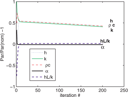
We bring this point up here because many heat transfer problems often behave as though they are functions of only a few groupings of variables, fewer than the apparent number of parameters in the model (this also occurs in our second problem discussed below) and are not well suited for inverse estimation because if converged solutions are obtained, it is only through a very large number of iterations. Such conditions appear to be ideal for using sparse grids because of their low computational costs, misleading the analyst as to their usefulness.

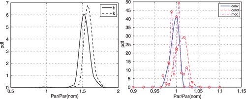
A serious practical problem in using the Bayesian approach is the need to define the parameter space over which the integration in Equation (7) will be conducted. Figure 2(a) shows the result using 11 Gaussian quadrature points sampling the range of each parameter from 1/2 the expected parameter value to twice the expected value with normally distributed priors for h, k and ρc. In this case of a simulated experiment, the expected values were set equal to the true values. Because only 2 parameters can be identified, only 2 unique pdf distributions are obtained. Once these initial distributions are known, it is common to refine the results by limiting the range of parameters. Figure 2(b) displays the results when sampling over the range of parameters from 0.9 to 1.1 times the expected values. We now find a very unusual pdf for ρc due to the ill-conditioning. For any given value of ρc, the temperature is a function of hL/k and thus there are multiple values of h and k that produce the same temperature history, i.e., the response surface is characterized by straight parallel contours giving a ripple effect. The consequent effect is that the peak of the pdf can be at any values of h and k that produce the same value of hL/k, thus the change from apparent maximum a posterior values in the neighbourhood of 1.5 to values closer to 1 and the generation of the strange pdf for ρc. If the cause of the strange results of Figure 2(b) is not known, the temptation would be to increase the number of Gaussian points and to repeat the calculations.

Figure 2. Effect of ill-conditioning on Bayesian inference for Problem 1.

Whether the problem is ill-conditioned or not, the need to set reasonable bounds on the parameter space for the Bayesian analysis suggests that one should first estimate the parameter values using the usual least-squares approach. This is especially relevant since the least-squares solution usually requires only a few evaluations of the model compared to the 1331 evaluations used to produce each of Figure 2.

For this first problem, if the ill-conditioning is not recognized, the poor performance of the least-squares solution often leads to the use of some form of regularization or the LM approach. Using the LM approach, one conducts a sequence of solutions, each using smaller values of the LM parameter, β. Convergence for any given value of β, if achieved at all, is reached very slowly. Figure 3 shows the history of the iterations for β = 0.01. Unfortunately h, k, ρc converged only for large values of β and led to incorrect results. Values of hL/k and α converged quickly, but h, k, ρc appear to be converging slowly, leading the analyst to continue iterating.

Figure 3. History of iterations using β = 0.01 for Problem 1 when ill-conditioned.

Table 1 lists the results as a function of β used in Equation (3a). N denotes the number of iterations needed to achieve converged values.

Table 1. Effect of β for σ = 1% (true values: k = 1.0,  h = 1.0, ρc = 20.0 Bi = 1.0, α = 0.05).

β	0.1	0.01	0.001
Bi	1.015	1.015	1.018
α	0.0494	0.0494	0.0493
N	14	14	10
k	1.480	1.408	0.0302
h	1.503	1.429	0.0308
ρc	29.96	28.49	0.6135
N	14	>200	Never

Problem 1

Well-conditioned results

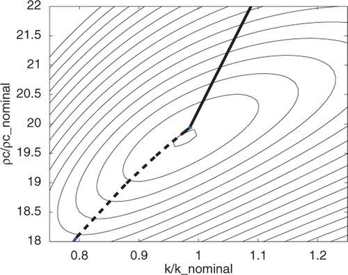
When the problem is well conditioned, the least-squares solution can be effected in a few iterations, of the order of 10, and there is little need to consider sparse grids. However, since we anticipate using sparse grids for the Bayesian approach it is of interest to see how well a least-squares approach based on evaluating M(Θ) in Equation (3a) using a sparse grid performs. Figure 4 compares the search trajectory when estimating only k and ρc from simulated data with 1% zero mean, random normally distributed noise. Two different starting points were used and the temperatures and sensitivities needed in Equation (3) were computed from the closed-form product solution 7 and by using a sparse grid. The paths for the sparse grid process are only slightly different than those from the exact solution and reach the same estimated values.

Figure 4. Solution trajectories for Problem 1 using exact solutions (solid line) and a sparse grid (dashed line) for two parameters of level 3 (29 sample points) for interpolation.

Problem 2

The second problem was a ‘real’ experiment in which a composite panel was heated with an electric blanket applied to its upper surface and cooled by free convection from the bottom surface and by forced convection from the stringer. Figure 5 is a cross-section of the panel. The goal was to estimate the heat losses from the upper and lower surfaces from temperatures measured with thermocouples attached to the surface and located as shown and from infrared thermograms of the upper surface.

Figure 5. Schematic of the panel (thermocouples are placed at the numbered points).

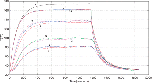
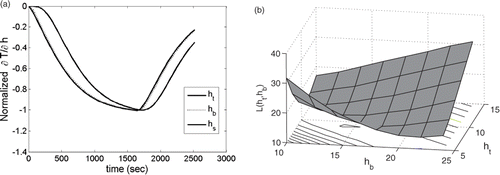
The panel was initially at room temperature and transiently heated by a constant current applied to the heating blanket. The heat losses, characterized by the convective coefficients, h_t, h_b, h_s for the panel top and bottom surfaces, and stringer surfaces, respectively, were estimated from the temperatures measured during heating as shown in Figure 6 plus the temperatures on the surface of the electric blanket as inferred from the infrared thermograms.

Figure 6. Time history of panel temperatures (numbers denote the thermocouples shown in Figure 5).

The panel temperatures needed in Equation (3) for the model M(x, t, h_t, h_b, h_s) were computed using the finite element multiphysics program Comsol 8. Figure 7 shows the trajectories of the least-squares solutions obtained using temperatures and sensitivities computed directly from Comsol and those from a sparse grid representation of the response surface.

Figure 7. Contours of L(Θ) showing the solution trajectories for Problem 2 using exact solutions of M(Θ) (–-) and interpolation by a sparse grid of level 3 (69 sample points) (- - -).

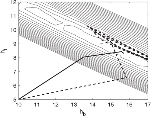
From the contours of L(Θ), Equation (2a), we see that the problem is ill-conditioned – the surface has many local minima and is too flat to unequivocally identify a global minimum. This is not unexpected since there are many combinations of the parameters that can lead to comparable results. For example, heat losses from the panel at thermocouples 7 and 10 are functions of h_t + h_b, not of their individual values and the response surface of M(Θ) is similar to that of Problem 1 with ripply contours. In this case the sparse grid interpolated values are so inexact that the sparse grid estimation never converges and simply wanders around the surface in an unpredictable way.

4. Sparse grid fundamentals

The idea behind sparse grids is very simple. Consider a function of two variables, f(x, y). The usual representation is through the Taylor series (13) Each term in this expansion represents a ‘complete polynomial’, i.e., the powers of x and y sum to a single value, e.g., the first term is a complete polynomial of power 0, the second of power 1, the third of power 2 and so on. Consider a tensor grid of sample points to represent the second-order expansion. In each direction, this will require three points, giving a total of nine points. However, there are only six constants that need to be evaluated. Thus one needs only six sample points. Of the three points on the diagonals, only one is needed, the remainder are superfluous. The question is ‘which diagonal point to choose and how to define an automatic procedure’ to choose it. In other words we can use a sparser grid than the tensor grid. Smolyak 9 developed a method that led to a high level of quality when interpolating and integrating functions. The method consists of combining different orders of 1D interpolation on nested spaces, i.e., sets of sample points for which the points of each set are intermediate to the points of the preceding set. The interpolating function is a set of linear combinations of products of the univariate polynomials. Each 1D interpolation is exact on certain nested spaces. Consider three sample points in each of the x and y directions, Figure 8(a). This will allow us to represent the univariate functions, f(x) = [1, x, x²], f(y) = [1, y, y²]. Smolyak's method represents f(x, y) by products of these univariate representations, i.e., f(x, y) = f(x)f(y). In this case we obtain f(x, y) = [1, x, y, x², xy, y², x²y, xy², x²y²].

Figure 8. Level 1 and level 2 sparse grid points: (a) level 1 points (O) and (b) level 2 additional points (X).

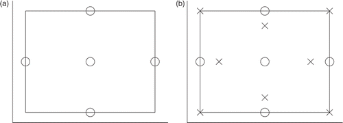
Obviously with the five sample points the product cannot represent all nine terms and we must eliminate some of the terms, giving f(x, y) = [1, x, y, x², y²], that is we filter the product solution. If we were to add eight (8) additional points as shown in Figure 8(b), the univariate function representations would be f(x) = [1, x, x², x³, x⁴], f(y) = [1, y, y², y³, y⁴], giving a product involving 25 terms. Of these, these sample points would allow only the determination of the coefficients for the following terms: (14) where l denotes the three grid levels used, l = 0, only the centre point, l = 1, the five points, l = 2, the 13 points. We see that only the first grid produces a complete polynomial, i.e., for l = 1, the term xy is missing. The missing terms are provided by the next higher level grid. But while l = 2 completes the lower order polynomial and adds more terms, it is lacking the terms to form a complete polynomial, i.e., for l = 2 we lack the two terms xy³, x³y. Smolyak's equation for f(x₁, … , x_d) can be written as (15) where i_j are the levels of the x_j grid and |i| = i₁ + ··· + i_d, where d denotes the dimensionality of the parameter space, denotes the univariate basis function in the jth dimension of level i and denotes the binomial coefficient = a!/(b!(a − b)!.

Smolyak's method did not attract much attention until Barthelmann et al. 10 demonstrated that the method was optimal. If we denote Smolyak's formula as 𝒜(q, d) where d is the number of dimensions and q denotes the level of interpolation, they proved that 𝒜(k + d, d) is exact for all complete polynomials of order d provided that nested grids are used and that the approximation is ‘best’ in that the error bounds are least. A sparse grid can be characterized by its ‘level’, essentially the order of the complete polynomial that can be interpolated. When using nested grids, each level contains the contributions of the lower levels.

A variety of sample point spacings may be used in the grids, but it is well known that using the Chebyshev knots leads to the min-max fitting which is almost as good as the best approximation possible.

Since Barthelmann's paper sparse grids have enjoyed increasing usage. Klimke 11 developed the program ‘spinterp’ which is available as a Matlab toolbox 12. Petras 13 describes efficient ways of computing the coefficients, Heiss and Winschel 14 have developed optimal formulae for Gaussian quadrature for likelihood functions, and a number of papers exist in which sparse grids are used for Bayesian inference and other problems of high dimensions 15–20.

5. Appropriate level of the sparse grid

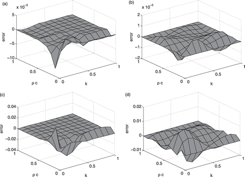
Because the number of sample points grows rapidly as the level is increased it is important to determine the appropriate level. Unfortunately this cannot be done in advance. One approach is based upon Klimke's sparse grid method based on ‘surpluses’ 11. A surplus is the amount each sample point contributes to the basis function, i.e., equal to the difference between the value of the function at the sample point, f(x_j) and the interpolated value at that point based upon the preceding level of the sparse grid. However the surplus is not a measure of a single sample point's contribution to the interpolation over the entire response surface, just at that point. Furthermore, the surplus can be determined only for scalar quantities, thus eliminating its use for the vectors and matrices used in the Bayesian inference. It is possible to determine the surpluses for a specific scalar, in our case the temperature at a given point in space and time. For the transient bar problem the temperature and sensitivities at x/L = [0, 0.25, 0.5, 0.75, 1.0] and αt/L² = [0 : 1 : 41] were calculated on the tensor grid defined by each parameter, h, k, ρc ranging from one half to twice its nominal value, i.e., 0.5 ≤ h, k ≤ 2 and 10 ≤ ρc ≤ 40 using 11 sample points in each dimension. The maximum and rms errors in the sparse grid interpolation at each of these tensor points was evaluated. The reduction in error as the sparse grid level was increased is shown in Figure 9 along with the estimated error from the program ‘spinterp’ evaluated at x/L = 0.5, Fo = 21. Similar comparisons made for other values of x and t gave comparable results. In almost all cases the estimated reduction in the maximum error based on surpluses was an underestimate of the increased accuracy as the sparse grid level was increased.

Figure 9. Reduction in maximum errors of T and ∂T/∂k as a function of sparse grid level for Problem 1 (maximum errors evaluated at x/L = [0, 0.25, 0.5, 0.75, 1.0], Fo = [0 : 1 : 41] (‘spinterp’ results evaluated at x/L = 0.5, Fo = 21).

Although Figure 9 suggests that in general that there was a monotonic behaviour as the sparse grid level increased, this was not always the case for every point studied. Figure 10 shows how the higher level sparse grid interpolations converge as a function of time for values of T and dT/dk at x = 0.5L. While the temperature is well represented for a grid of level 3, ∂T/∂k requires a minimum of level 5 for good representation over entire range of times.

Figure 10. Interpolated values for sparse grids of increasing levels for Problem 1 using the Chebyshev grid (numbers denote the level): (a) T at x/L = 0.5, Fo = 21 and (b) ∂T/∂k at x/L = 0.5, Fo = 21.

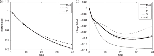
An additional option when using sparse grids is the choice of the grid. The most common are those based on Chebyshev polynomials, the Clenshaw–Curtis grid and the Patterson grid. Figure 11 shows that while the interpolated temperatures are similar, the convergence for ∂T/∂k differs between the different grids.

Figure 11. Interpolated values for sparse grids of increasing levels for Problem 1 using the Clenshaw–Curtis grid (numbers denote the level): (a) T at x/L = 0.5, Fo = 21 and (b) ∂T/∂k at x/L = 0.5, Fo = 21.

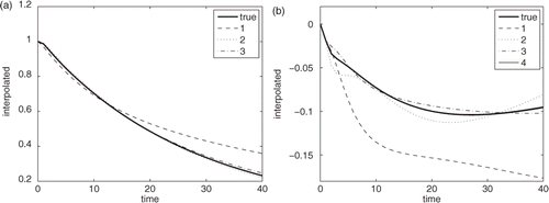
When solving the estimated parameters using the least-squares approach for well-conditioned problems, inaccuracies in estimating the sensitivities are not of paramount concern, since these erroneous values simply result in non-optimum trajectories in the parameter space. A more critical concern is the accuracy of representation of the quantity being fitted, in our case, temperatures. Figure 12 compares the errors over the tensor grid for parameters k and ρc for the temperature and for ∂T/∂k. Although the errors are less for the Chebyshev grid, the tendency of the Chebyshev polynomials to manifest errors as ripples can cause problems as we will see in the discussion of the second problem, the real experiment.

Figure 12. Interpolation error for the temperature at x/L = 0.5, Fo = 21, Problem 1: (a) Clenshaw–Curtis grid and (b) Chebyshev grid. Interpolation error for the ∂T/∂k at x/L = 0.5, Fo = 21, Problem 1: (c) Clenshaw–Curtis grid and (d) Chebyshev grid.

6. The use of sparse grids in fitting ∂T/∂k versus differencing T

Sparse grids can be represented in two ways: (a) the method introduced by Klimke based on surpluses and available in the Matlab 12 toolbox, ‘spinterp’, (b) an approach utilizing basis vectors described by Agarwal and Aluru 21. ‘spinterp’ treats only scalar values and for inverse problems it is not the best approach. Agrawal and Aluru constructed the basis vectors as follows.

Let the interpolation over all of the N_sp sample points of the parameters, Θ be expressed as (16) where are the coordinates of the different parameters, f(Θⁱ) are the values of the model at these points and L_i(Θ, Θ_i) with L_i(Θ_j, Θ_i) = δ_ij are the basis functions. We construct the basis function L_i(Θ, Θ_i) by adding the contributions from all the sampled values. Consider evaluating the model M(Θ, x_α, t_j) at a number of spatial positions x_α and times t_j. For each set of parameter values, Θⁱ, the model response can be assembled in a matrix with elements Rⁱ(x_α, t_j) and the interpolated value at any point Θ* is then given by (17) where ℛ is a vector of length N_sp whose elements are the individual matrices Rⁱ(x_α, t_j) and ℒ is a column vector (the multiplication in Matlab is done by defining ℛ and ℒ as cells).

In estimating the parameters using the least-squares approach we need the sensitivities, ∂T/∂k. We have a number of choices: first using exact solutions of M(Θ): (a) compute the sensitivities from the appropriate partial differential equation, or (b) finite difference the temperatures; second to obtain the temperature and sensitivity by interpolation of their respective response surfaces using the sparse grid; third by using the sparse grid representation of the temperature to obtain the sensitivities by (c) finite differencing the interpolated temperatures or (d) to differentiate the temperature interpolating polynomials.

Recognize that the univariate polynomial is represented as 22 (18) where (19) (20) a_ν, b_μ are the sample points. Differentiating f(x, y) will require evaluating n(n − 1)m(m − 1) functions. Even for relatively few sparse grid points, this turns out to be too expensive. If the sparse grid interpolation of the temperature is reasonably exact, then one should do as well by finite differencing the interpolated values. When this suffices, we term the sparse grid interpolation to be ‘well conditioned’. Figure 13 compares the trajectories by the three different methods.

Figure 13. Trajectory for different ways of determining the sensitivities: Exact, solving using the model; SG-a, finite differencing interpolated temperatures; SG-b, differentiating interpolating polynomials representing temperature; SG-c, interpolating sensitivities.

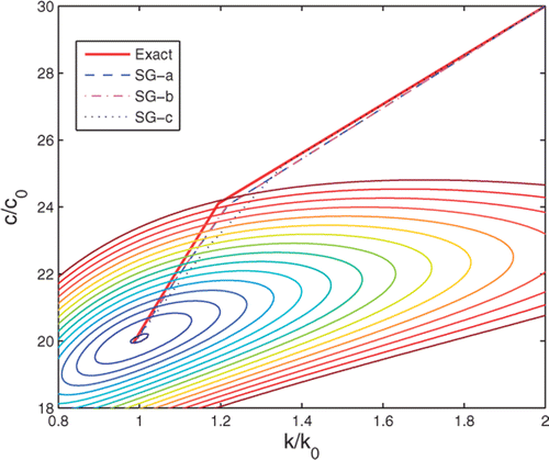
Method SG-b, as noted above is far too expensive and when the temperature is well fitted is no better than finite differencing the interpolated temperatures, method SG-a. On the other hand, the errors observed in representing the sensitivities as shown in Figures 10(b) and 11(b), lead to a different trajectory, but the same final estimate.

7. Bayesian inference – need for good values of and

Given that for most problems that we may not have a good idea of the parameter values or even the resulting estimates, , one often chooses a rather large range within which to locate the initial estimate in solving Equation (3a) or for obtaining the pdfs in the Bayesian approach. For these two example problems we assumed that the parameters would be in the range of 0.5 * θ_nominal to 2 * θ_nominal where the ‘nominal’ value was a very intuitive guess. For many problems, the model response near the extreme parameter values is often much different than that at the final estimated parameter values. This leads to two problems: (1) the sparse grid errors are greatest at these points, Figure 11; (2) the pdfs obtained from the Bayesian approach are markedly affected. Figure 14(a) shows the pdf for the conductivity obtained using a non-informative prior and 41 Gaussian quadrature points on a tensor grid (1681 points) as compared to the pdf based upon the least-squares procedure. The maximum a posterior value is much displaced from that estimated by least-squares and the uncertainty is substantially larger. The primary problem is that the sample points are spaced too far apart and the peak pdf is not captured well. A reasonable depiction of the pdf requires 2–3 points to be sampled in the region to . For many inverse problems, especially those involving actual experiments, is of the order of 10% in order to capture the maximum a posterior probability a reasonable number of points is needed around the maximum point. When sampling over the range 0.5 ≤ Θ/Θnom ≤ 2 this may require more than 21 Gauss-Legendre quadrature points because of their non-linear spacing. Such a large number of points is computationally unattractive. The solution, of course, is to use sparse grid interpolation and to compute the pdf over a smaller range – at minimal cost. Figure 14(b) displays the pdf computed by interpolating using a sparse grid of level 3 (29 points) with 41 quadrature points centred about the least-squares estimate of k. The two distributions are nearly identical, with differences only in the tails.

Figure 14. Effect of refining the range of parameters for in Problem 1 (ρc specified): (a) expanded range and (b) centred about LS solution using sparse grid interpolation.

8. Ill-conditioned problems and the use of sparse grids

Classically, ill-conditioning occurs when two or more of the sensitivities used in Equation (3a) are very similar to each other, leading to a nearly zero determinant. This occurs in Problem 1 where the temperatures are functions only of two parameters, Bi = hL/k and α = k/ρc and all three parameters are sought. In this case the source of the ill-conditioning was easy to identify and anticipate. For the panel problem, the three convective coefficients h_t, h_b, h_s are not similarly related, but the physics of the actual heat transfer makes it difficult to separate their effects. In the centre of the panel, near locations 8 and 10, the heat loss is by convection from the top and bottom surfaces, i.e., ∝(h_t + h_b) and their effects cannot be determined individually. Because the in-plane conductivity is so much higher than the out-of-plane conductivity, the temperature at location 9 is affected by the loss from the bottom surface and from the stringer, that is ∝(h_t + C₁h_b + C₂h_s) where C₁ and C₂ are constants. As a consequence the sensitivities of the temperature at this location to the three coefficients are very similar, Figure 15(a). Although the sensitivities at other points were not so equal, the problem is very ill-conditioned with the surface L(Θ) being very flat as shown in Figure 15(b) and possessing several local minima. The inaccuracies inherent in the sparse grid approximations in representing the behaviour near the minimum value of L(Θ) make finding the global minimum very difficult as shown in Figure 7.

Figure 15. Behaviour of the panel: (a) time history of sensitivity of temperature and (b) surface of L(h_t, h_b) for the panel at TC 9.

9. Conclusions

Calculating the marginal probability distribution from Equation (7) requires a fairly dense sampling of the integrand near the point of maximum probability and, if using a sparse grid a reasonable level of accuracy. For the problems considered here, and true in general, the response surface shows some strong variations near the corners of the parameter space, Figure 12. Consequently it is important to choose the smallest parameter ranges possible. Although the maximum a posteriori probability may not coincide with the estimated value of from the least-squares analysis, , we have found that defining the range of each parameter to be where is given by Equation (3c) and n is a small number, usually 4 or 5, suffices. The advantage of the sparse grid (or of any other interpolation) is that locating the peak probability and the effect of assuming different priors in Equation (7) can be examined with minimal computational expense. For the panel, computing the time history for a given set of parameters required in the order of 65 s compared to 0.8 s when using the sparse grid of level 5.

Our recommended procedure is:

1.	determine with the least-squares approach using the model M(Θ, x, t),
2.	define the parameter space based upon ,
3.	develop the sparse grid interpolation for levels l1–lm: a. at each level choose some representative responses and use ‘spinterp’ to evaluate the maximum surplus as a measure of the accuracy of the sparse grid, b. compare the behaviour of the sparse grid representation of these points with their actual performance, as in Figure 10, c. choose the appropriate maximum level, lM based upon the surpluses and 3(b),
4.	use the sparse grid to calculate the marginal pdf.

The choice of the representative points in 3(a) must be made with some care to ensure that a good agreement is not fortuitous or unrepresentative of the interpolation accuracy over the entire parameter space. If the comparison is of the transient behaviour, then although N responses at T times will involve NT calls to ‘spinterp’, these computations are cheap.

While, as in the examples presented here, one can generate the sparse grid values on a reasonably large parameter space and use sparse grid interpolation to determine and , and then proceed directly to step 4, an initial guess using least-squares, even for poorly conditioned problems, can often be obtained with only a few model evaluations giving a much better definition of the parameter space to be used in step 3.

Besides reporting the surpluses ‘spinterp’ can provide information about adaptive grids, i.e., grids with different numbers of sample points in each dimension. While this may reduce the number of sample points needed, special care must be taken to ensure that the interpolation is accurate over the entire parameter space. Although Equation (7) involves only interpolation of the response, we have found that good interpolation of the sensitivities rather than just of the response is a better measure of the sparse grid acceptability.

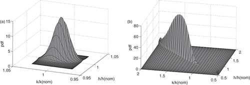
Ill-conditioned parameter estimation problems are usually identified by the behaviour of the matrix (A^TΣ⁻¹A) in Equation (3). The ill-conditioning usually arises when the sensitivities for two or more parameters are nearly equal. For some problems it is possible to compare the sensitivities and understand why they are so alike. However, for many problems such causes are not easily discerned. For the panel problem some temperatures showed similar sensitivities, but others did not. Sparse grids can be used to detect the cause of the ill-conditioning. Figure 16(a) shows the joint probability density of h and k when ρc is fixed. Since both h and k appear in the Biot number, there is a reasonably high correlation between their estimated values, but the joint pdf is reasonable. When all three parameters are sought, the joint pdf for any pair of parameters shows very unusual effects, Figure 16(b). Here the ill-conditioning shows up as abrupt rises and falls in the pdf (the dark vertical triangles) and in the extreme thinness. We have found similar behaviour in other problems where the parameters occur in non-dimensional groups.

Figure 16. Joint probability densities for Problem 1: (a) well-conditioned and (b) ill-conditioned.

These conclusions are valid only for well-conditioned problems. For the panel test, the values of were of the order of 15% and an adequate coverage of the parameter space needed for an accurate evaluation of Equation (7) required interpolation over such a wide range of parameters and responses, Figure 12, that reasonable levels of sparse grid were not a viable option. In fact, for such ill-conditioned problems it is questionable whether evaluating the marginal pdf is of any value unless one is specifically interested in the tails of the distribution, e.g., reliability studies.

Acknowledgements

A portion of this research was conducted under the sponsorship the Washington State Technology Center, contract RTD09 UW GS09, the United States Federal Aviation Administration Cooperative Agreement 08-C-AM-UW and the National Science Foundation, Grant 0626533. We thank Professor N.R. Aluru and Doctoral candidate, N. Agarwal for the initial Matlab version of the sparse grid basis program.

References

- Press, WH, Flannery, BP, Teukoslky, SA, and Vetterling, WT, 1986. Numerical Recipes. Cambridge: Cambridge University Press; 1986.
- Seber, GAF, and Wild, CJ, 1989. Nonlinear Regression. New York: Wiley & Sons; 1989.
- Shiavi, R, 1999. Introduction To Applied Statistical Signal Analysis. New York: Academic Press; 1999.
- Bolstad, WM, 2004. Introduction to Bayesian Statistics. New York: Wiley & Sons; 2004.
- O'Hagan, A, and Forster, J, 2004. Bayesian Inference, Kendall's Advanced Theory of Statistics. Vol. 2b. Oxford: Oxford University Press; 2004.
- Gelman, A, Carlin, JB, Stern, HS, and Rubin, DB, 2004. Bayesian Data Analysis. Boca Raton, FL: Chapman & Hall/CRC Press; 2004.
- Carslaw, HS, and Jaeger, C, 1959. Conduction of Heat in Solids. Oxford: Clarendon Press; 1959.
- COMSOL, Version 3.5a, Heat transfer module user's guide, COMSOL Multiphysics, 2008.
- Smolyak, S, 1963. Quadrature and interpolation formulas for tenser product of certain classes of functions, Sov. Math. Dokl. 4 (1963), pp. 240–243.
- Barthelmann, V, Novak, E, and Ritter, K, 2000. High dimensional polynomial interpolation on sparse grids, Adv. Comput. Math. 12 (2000), pp. 273–287.
- Klimke, A, , 2008. Sparse grid interpolation toolbox user's guide; available at www.ians.uni-stuttgart.de/spinterp/download.htm.
- MATLAB version 7.1.0., The Mathworks Inc., Natick, MA.
- Petras, K, 2001. Fast calculation of coefficients in the Smolyak algorithm, Numer. Algor. 26 (2001), pp. 93–109.
- Heiss, F, and Winschel, V, 2008. Likelihood approximation by numerical integration on sparse grids, J. Econ. 144 (2008), pp. 62–80.
- Achatz, S, 2003. Higher order sparse grid methods for elliptic partial differential equations with variable coefficients, Computing 71 (2003), pp. 1–15.
- Garcke, J, and Hegland, M, 2009. Fitting multidimensional data using gradient penalties and the sparse grid combination technique, Computing 84 (2009), pp. 1–25.
- Gerstner, T, and Griebel, M, 2008. Sparse Grids: Encyclopedia of Quantitative Finance. New York: Wiley & Sons; 2008.
- Ma, X, and Zabaras, N, 2009. An adaptive hierarchical sparse grid collocation algorithm for the solution of stochastic differential equations, J. Comput. Phys. 228 (2009), pp. 3084–3112.
- Ganapathysubramanian, B, and Zabars, N, 2007. Sparse grid collocation schemes for stochastic natural convection problems, J. Comput. Phys. 225 (2007), pp. 652–685.
- Lin, B, and Tartakovsky, AM, 2009. An efficient, high-order probabilistic collocation method on sparse grids for three-dimensional flow and solute transport in randomly heterogeneous porous media, Adv. Water Resources 32 (2009), pp. 712–722.
- Agarwal, N, and Aluru, NR, 2009. Stochastic analysis of electrostatic MEMS subjected to parameter variations, J. Microelectromech. Syst. 18 (2009), pp. 1454–1468.
- Steffensen, JF, 1950. Interpolation. New York: Chelsea; 1950.