On the Laplacian operation with applications in magnetic resonance electrical impedance imaging

Abstract

Consider the numerical computation of Laplacian operation from the noisy data of a given function f(x) defined in Ω ⊂ ℝ². By expressing this ill-posed problem as a Fredholm integral equation of the first kind, we construct the approximate solution from a PDE boundary value problem directly, which can be considered as the Lavrentiev regularization in essence. The optimal error estimate of this regularization for an appropriate a posteriori choice strategy of the regularization parameter is given under some source conditions of the exact Laplacian operation. An iterative algorithm for computing this a posteriori regularization parameter under the framework of model function method is also given with its convergence analysis. The advantage of the proposed scheme is that we treat the Laplacian operation as a whole, rather than the partial derivatives of each variable, and therefore the Laplacian operation can be computed in a bounded domain with arbitrary boundary shape for noisy data specified at randomly scattered points. At last, we apply this scheme to the iterative algorithm of reconstructing the conductivity in magnetic resonance electrical impedance tomography, where the input data is the magnetic flux data for which the Laplacian operation must be carried out. The validity of the proposed scheme is shown numerically for this new medical imaging technology.

Keywords:

• Laplacian operation
• ill-posedness
• regularization
• MREIT
• convergence
• numerical solution

1. Introduction

Numerical differentiations are classical ill-posed problems which have been researched extensively, with the aim of computing the derivatives of a function stably from its given noisy data. It was understood long time ago, for example see 1,2, that the step size in the difference scheme of numerical computation can be taken as the regularization parameter for given noisy data, i.e. the difference step should be chosen in terms of the error level of the noisy data appropriately. For numerical differentiations of the functions defined in ℝ¹, there have been so many works in the past years, for example see 3–7, while the applications of such kind of problems can be found in the Dupire formulae in financial mathematics 8,9, image edge detection 10,11, solvability of the Volterra equation of the first kind 12 and so on.

Compared with numerical differentiations of the functions defined in ℝ¹, the same problems for f(x) with x = (x₁, x₂, … , x_n) ∈ ℝⁿ (n ≥ 2) are not so well-researched mathematically, while such kind of problems arise in applied areas extensively. Although, these problems can be considered as the partial derivatives of each independent variable x_i in principle, such a direct mathematical consideration will lose some special physical structure of the given applied problems. In fact, the differential operators for f(x) defined in ℝⁿ arising in applied areas are often of some special peculiarity, not merely the computations of partial derivatives. For example, the Laplacian Δ or double Laplacian Δ² often appear in mechanics. On the other hand, the points specifying the noisy input data may be randomly scattered, therefore the numerical differentiation using standard difference scheme for such input data is impossible. Finally, the domain Ω ⊂ ℝⁿ for n ≥ 2, where the numerical differentiation is sought, may be of arbitrary boundary shape ∂Ω. In this case, similarly to solving the direct PDE boundary value problem by difference scheme, the irregular boundary shape may cause some difficulty in the mesh generation. Thus, the numerical differentiation problems in higher dimensional cases should be treated carefully.

Based on the above considerations from the engineering situations, and also motivated by our recent works on the medical imaging technology using the magnetic resonance electrical impedance tomography (MREIT) 13,14, the purpose of this article is to consider the stable computation of the Laplacian operation in an arbitrary bounded domain Ω ⊂ ℝ². In the recently developed harmonic B_z algorithm of MREIT, the reconstruction of the conductivity distribution of a 3-dimensional biological tissue is done in all the 2-dimensional slices. This algorithm constructs an iterative formula for the conductivity σ(x, y, z₀) at each slice {z = z₀}, where the Laplacian operation Δ_x,yB_z(x, y, z₀) for the given z-component of the magnetic flux density B_z(x, y, z₀) is taken as the input data. The harmonic B_z algorithm had been proved to be of higher accuracy for exact data B_z. However, to make this algorithm implementable for measurement data B_z, we must consider the noisy data of B_z in an arbitrary tissue domain Ω ⊂ ℝ². In this case, the crucial problem is the numerical approximation of ΔB_z from the noisy data in Ω.

For treating ill-posed problems, both the construction of regularizing schemes and the error estimate of the regularizing solution play important roles. More precisely, the error estimate depends on the choice strategy of the regularizing parameter in terms of the error level of the input noisy data. In the case of seeking derivatives of the functions defined in ℝ¹, many regularizing schemes have been proposed. Hanke and Scherzer 3, gave a successful analysis for treating numerical differentiation by the Tikhonov regularization, where the error estimate of the regularizing solution was given by using the discrepancy principle to choose the regularizing parameter. The idea of 3 was extended to treat the numerical differentiation on irregular grids in 7, and the authors gave a very simple strategy for choosing the regularization parameter. A simple scheme for stable numerical differentiation of given noisy data was proposed in 15 by expressing the differentiation as a solution of an integral equation of the first kind, then the Lavrentiev regularization was introduced and the convergence analysis of the regularizing solution was also given in 15. For the higher order derivatives of the function defined in ℝ¹ and the partial derivatives of the function defined in ℝ², stable numerical differentiation schemes can be found in 16–19 and references there in.

Motivated by the successful work in 3,15,19, we reformulate the computation of Laplacian operation in a bounded domain Ω ⊂ ℝ² as the solution of a Fredholm integral equation of the first kind, using the Green function of the Dirichlet problem for the Laplace equation as the integral kernel. However, we do not regularize this ill-posed integral equation A[u] = f by the Tikhonov regularization, noticing the large amount for computing the A*A in 2-dimensional domain. Instead, we construct a boundary value problem for a PDE with small parameter α to approximate the original problem, which can be considered as the Lavrentiev regularization in essence. However, this PDE-based version of the regularization enables us to capture the regularizing solution in a direct way. The optimal error estimate of the regularizing solution for an appropriate a posteriori choice strategy of the regularization parameter is given in this article under the source condition of the exact solution. Furthermore, a numerical iterative algorithm for computing the a posteriori regularization parameter is also given with its convergence analysis. From the numerical point of view, the regularizing solution defined from a boundary value problem in a bounded domain enables us to use some standard software such as PDE Toolbox in Matlab to get the numerical solution easily. At last, an application of our scheme for computing the Laplacian operation in MREIT is given, which shows the validity of the proposed scheme.

The outline of this article is as follows. In Section 2, we reformulate the computation of Laplacian operation as the solution of a Fredholm integral equation of the first kind and approximate its solution by a PDE boundary value problem. Under the source condition of the exact solution, the optimal error estimate of the regularizing solution for an a posteriori choice strategy of the regularization parameter is given in Section 3. An iterative algorithm for computing the a posteriori choice strategy of the regularization parameter with its convergence analysis is given in Section 4. This new iteration scheme essentially belongs to the category of recently developed model function method. In Section 5, some numerical examples are given for showing the validity of our scheme. At last, an application of our scheme in MREIT for reconstructing the conductivity is given in Section 6, where the Laplacian operation of the noisy magnetic flux data is input data.

2. The stable computation of Laplacian operation

Suppose that Ω ⊂ ℝ² is a simply connected bounded domain with piecewise smooth boundary ∂Ω. Let f ∈ H²(Ω) be a given real-valued function, u = Δf ∈ L²(Ω) is its Laplacian operation. Without loss of generality, we assume f |_∂Ω ≡ 0, otherwise the function f(x) ≔ f(x) − f₀(x) with f₀(x) solving (1) satisfies f |_∂Ω = 0 and Δf = u.

Denote the Green function of the Dirichlet problem for the Laplace Equation in ℝ² as where g(x, y) is a harmonic function in Ω and has the same boundary value with on ∂Ω. Then the relation between f and u can be expressed as (2) Obviously, the operator A is linear in L²(Ω). Further, we have the following result, where the norm ‖·‖ and the inner product ⟨·, ·⟩ without subscript are in L² sense.

Lemma 2.1

The operator A: L²(Ω) → L²(Ω) is nonnegative, self-adjoint and compact.

Proof

Since for all u ∈ L²(Ω) satisfying A[u] = −f, it has the operator A is nonnegative in L²(Ω).

For all u, v ∈ L²(Ω) satisfying A[u] = −f and A[v] = −g, it has Thus, the operator A is self-adjoint in L²(Ω).

For the integral operator A, its kernel G(x, y) is weakly singular in {(x, y) ∈ Ω × Ω | x ≠ y}, since the function is weakly singular and g(x, y) is continuous in {(x, y) ∈ Ω × Ω | x ≠ y}. Thus, the operator A: L²(Ω) → L²(Ω) is compact, see 20.▪

The operator equation (2.2) is ill-posed, since the operator A is compact and its range R(A) = { f ∈ H²(Ω) | f |_∂Ω = 0} is infinite-dimensional, see 20. Consider the noisy data f^δ ∈ L²(Ω) satisfying (3) where δ > 0 is the error level. Our purpose is to compute the approximation of u = Δf from f^δ, which is equivalent to solve the operator equation (2.2) from f^δ. Some regularization methods should be introduced, as the equation A[u] = −f^δ is ill-posed. Since the operator A is nonnegative, the Lavrentiev regularization, or sometimes, the simplified regularization is applicable, see 21–25 for its general theoretical framework. The approximate solution for this regularizing scheme is computed from (4) where α > 0 is the regularization parameter. The standard results of the Lavrentiev regularization show that the operator equation (2.4) has a unique solution u^α,δ ∈ L²(Ω) and lim_δ→0 u^α(δ),δ = u, provided that α = α(δ) be chosen such that (5) However, the expression (2.5) can not give a quantitative choice of α in terms of δ, also the convergence rate of the regularizing solution u^α(δ),δ may be arbitrarily slow. In order to get its convergence rate, some choice strategies of α = α(δ) should be introduced based on some a priori assumptions of the exact solution u = Δf. There have been so many choice strategies of the regularization parameter α = α(δ) in the literatures 21–30 and the references therein. Some of them will be discussed in the next section.

As the kernel function G(x, y) of the operator equation (2.2) can not be known for an arbitrary 2-dimensional domain Ω, the regularizing equation (2.4) can not be solved directly, thus, we propose to solve (2.4) from an equivalent PDE boundary value problem numerically. Define h^α,δ ≔ A[u^α,δ], then it follows from the definition of operator A that Therefore, (2.4) becomes (6) with (7) From this boundary value problem, we can compute h^α,δ(x) in Ω by some numerical methods and finally get (8) From this expression, we see that the item takes the effect of regularization. Using this item to filter out the noise of , we can get the stable numerical scheme. However, h^α,δ(x) = 0 for x ∈ ∂Ω and the regularizing solution only relies on the value of f^δ(x). That is, there is no regularization on ∂Ω. In fact, the effect of regularization has been weakened when x is close to ∂Ω, thus we can only ensure that the regularizing solution is satisfactory in the interior part of Ω.

3. The choice of regularization parameter α

In order to get the convergence rate of the regularizing solution u^α,δ, some a priori assumptions of the exact solution u = Δf are needed. In general, the source condition u ∈ R(A^v), v > 0 is exploited, where the fractional power for the self-adjoint operator A and is its spectral decomposition. By choosing the regularization parameter α = α(δ) appropriately, the optimal convergence rate ‖u^α,δ − u‖ = O(δ^v/(v+1)) holds under the source condition when 0 < v ≤ 1, see 25,30. There have been several parameter-choice strategies that can ensure the optimal convergence rate of the regularizing solution u^α,δ. Among them, the a priori choice strategy is α(δ) = cδ^1/(v+1) 24, the modified discrepancy principle 25,27 or the generalized Arcangeli's method 22,26,29 belongs to the a posteriori choice strategies.

For the ill-posed problem A[u] = −f^δ in the last section, the a priori choice strategy α(δ) = cδ^1/(v+1) is hard to be applied in practice, since the determination of constant c relies on the a priori assumption of u. Compared with the a priori choice strategy, the a posteriori choice strategy only relies on the noisy data and its noise level in general, therefore, is more useful. Among the a posteriori choice strategies, the modified discrepancy principle is to choose the regularization parameter α = α(δ) by solving the nonlinear equation (9) This equation has a unique solution α = α(δ) provided that Cδ < ‖ f^δ‖, then the convergence rate of the regularizing solution u^α(δ),δ is optimal under the source condition u ∈ R(A^v), 0 < v ≤ 1. The generalized Arcangeli's method is to choose α = α(δ) by (10) The optimal convergence rate of u^α(δ),δ holds under the source condition by taking p = (q + 1)/(v + 1) in (3.2).

A novel a posteriori choice strategy of the parameter α = α(δ) is the generalized discrepancy principle, which needs to solve (11) This equation has a unique solution α = α(δ) provided that δ < Cδ^γ < ‖ f^δ‖. The convergence of the regularizing solution u^α(δ),δ had been shown in 19,31. However, the optimal convergence rate of u^α(δ),δ under the source condition is still unknown. In the next theorem, we will give an a posteriori error estimate which leads to the optimal convergence rate when smoothness v of the unknown solution is known.

Theorem 3.1

Assume that u ∈ R(A^v), 0 < v ≤ 1. Let C > 0 and 0 < γ < 1 satisfy δ < Cδ^γ < ‖ f^δ‖ and α = α(δ) be chosen according to (3.3). Then (12) Further, if v is known in advance, then for the choice of γ ≔ 1/(v + 1), the optimal convergence rate (13) holds.

Proof

Assume that u = A^v[w], w ∈ L²(Ω), 0 < v ≤ 1, then it has (14) where u^α is the regularizing solution with f^δ replaced by the exact data f in (2.4), see 25.

Notice that Hence, (15)

On the other hand, it has (16) where ‖u^α‖ = ‖(αI + A)⁻¹A[u]‖ ≤ ‖u‖ is applied. Inequality (3.8) and α‖u^α,δ‖ = ‖A[u^α,δ] + f^δ‖ = Cδ^γ yield i.e. . Therefore, it has (17) For δ is small enough, the convergence rate (3.4) follows from (3.6), (3.7) and (3.9). The choice of γ = 1/(v + 1) leads to the optimal convergence rate (3.5).▪

Remark 3.2

The best convergence rate O(δ^1/2) of the regularizing solution u^α,δ is achieved for u ∈ R(A) when γ = 1/2. In addition, the conclusions of the theorem can be extended to the operator equations with compact operator A which is just nonnegative, not self-adjoint.

When the parameter α = α(δ) is chosen by the generalized discrepancy principle, the nonlinear equation (3.3) with respect to α needs to be solved for given constants C and γ satisfying δ < Cδ^γ < ‖ f^δ‖. Therefore, we will propose an iterative algorithm for solving this nonlinear equation numerically in the next section.

Remark 3.3

Our proposed method depends upon knowing δ and C, both of which have to satisfy certain restrictions. It should be noticed that the noise level δ may be unknown from real data. Therefore, it is preferable to give some method to estimate δ from the measurement data f^δ itself. Fortunately, there are already some work on this direction which gives a lower bound on δ by iteration process, see 32. On the other hand, we also need that the positive constant C satisfies δ < Cδ^γ < ‖ f^δ‖, which is equivalent to . In the case of experimental data f^δ, this assumption can be met for specific C > 0 chosen in some typical way. For example, if we assume that 0 < δ < 1 (small noise) and , then we can always take C = 1. The assumption means that the amplitude of the measurement data should be larger than the noise level, which is quite natural from practical situation, otherwise the data will be completely contaminated by the noise.

4. Numerical computation of the regularizing parameter

Define then Equation (3.3) can be rewritten as H(α) = 0. From the derivation procedure in 19, it has An efficient scheme for solving the nonlinear equation H(α) = 0 is based on the idea of model function method to determine a regularizing parameter sequence {α_k : k ∈ ℕ} to approximate the exact zero point of H(α). More precisely, we construct a function h_k(α) of explicit analytic expression with finite number of parameters, which is taken as local approximation to H(α) near α_k. The finite number of parameters in h_k(α) are updated at each iteration step, then the zero point of h_k(α) is considered as α_k+1. Of course, different form of h_k(α) yields different model function. For more details about model function method, the readers can refer to 32–34.

Consider the nonlinear equation H(α) = 0, we utilize a linear function with single parameter to approximate H(α) locally, where C is the constant in H(α) and D needs to be updated at each iteration step. In the next, we will introduce a renewed iterative algorithm for D, which makes h(α) to be a local approximation to H(α), then the zero point of h(α) = 0 approximates the exact solution α* of H(α) = 0 by iteration. The iterative algorithm is given as follows, where the bisection method is embedded in order to guarantee the convergence of iteration sequence.

Give initial guess α₀ > 0 satisfying H(α₀) > 0, tolerance level ϵ > 0 and set k = 0.

	Step 1 Solve Equations (2.6)–(2.8) to generate .
	Step 2 Compute Dk from the requirement hk(αk) = H(αk), which yields (18) hence, the k-th approximate function of H(α) near αk is (19)
	Step 3 The zero point of hk(α) is (20) If H(αk+1) = 0, stop, or if H(αk+1) > 0, goto Step 4; otherwise set recursively until H(αk+1) > 0 and go to Step 4.
	Step 4 If |αk+1 − αk| ≤ ϵ, stop; otherwise take k ≔ k + 1 and go to Step 1.

The validity and convergence analysis of this iterative algorithm are given as follows.

Theorem 4.1

Let α₀ > α*, the above iterative algorithm generating sequence {α_k} either

1.	stops at αK = α* with the finite iteration step K; or
2.	is infinite, monotone decreasingly and converges to α*.

Proof

We divide the proof as two parts.

Part 1 The existence of sequence {α_k : k ∈ ℕ}.

If H(α_k+1) > 0 holds in Step 3, then α_k+2 can be determined obviously from the algorithm. Also, it follows 0 < α_k+1 < α_k from h_k(α_k+1) = 0 and the facts Let us consider the case H(α_k+1) ≤ 0 appearing for the first time in Step 3, then it has H(α_k) > 0. Without loss of generality, it is enough to consider H(α_k+1) < 0, otherwise α_k+1 = α* has already been the exact zero point of H(α), which is just the first case of the theorem. Since H′(α) > 0, it follows that α* ∈ (α_k+1, α_k). Noticing 0 < α_k − α_k+1 < α₀, the finite number of bisection recursions make α_k+1 ∈ (α*, α^k), which implies that H(α_k+1) > H(α*) = 0, and α_k+2 can also be generated from the iterative algorithm. Thus, the sequence {α_k} is infinite and monotone decreasingly.

Part 2 The sequence {α_k} converges to α*.

Since the sequence {α_k} is monotone decreasingly with lower bound α* > 0, it of course converges as k → ∞. Denote , we need to prove , which is equivalent to due to the uniqueness of H(α) = 0. From the definition of h_k(α), it has From the proof of Theorem 3.1, we know that This and the convergence of {α_k} generate Hence, it has from the continuity of H(α) and the update of {α_k}.▪

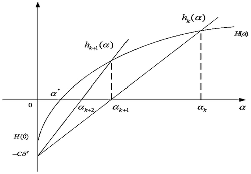
By utilizing a linear function h(α) to approximate H(α) locally, we get an effective iterative algorithm to solve the generalized discrepancy principle. Its essence is shown in Figure 1. This algorithm is similar to the secant method for solving nonlinear equation. Due to the value of H(0) which cannot be gotten in advance, we use −Cδ^γ to approximate it.

Figure 1. The approximation to α* by above iterative algorithm.

In fact, the above iterative algorithm can also be used to solve the modified discrepancy principle and the generalized Arcangeli's method given in the last section. For the modified discrepancy principle, we need to solve the nonlinear equation M(α) = 0, where (21) For the operator equation A[u] = −f^δ, it has 25 For the generalized Arcangeli's method, the nonlinear equation G(α) = 0 need to be solved, where (22) Then, it has 22 Similar with the above iterative algorithm for solving the generalized discrepancy principle and its convergence analysis, we can get the corresponding iterative algorithm for solving both the above a posteriori choice strategies.

5. Numerical examples

In this section, we will give some numerical examples to show the validity of our scheme for computing the Laplacian operation with the a posteriori choice strategies of the regularization parameter.

Example 1

Consider the function (23) then it has u = Δf = −2π²f. Take the noisy data of f(x, y) as where rand is a random number in (−1, 1). Since f |_∂Ω ≡ 0, the regularizing solution u^α,δ can be computed from (2.8) directly, where the boundary value problem (2.6)–(2.7) can be solved by the PDE Toolbox in Matlab. The regularization parameter α = α(δ) is chosen by the a posteriori choice strategies where the iterative algorithm given in the last section is occupied with α₀ = 0.1 and ϵ = 10⁻⁶. The regularization parameters chosen by the generalized discrepancy principle (3.2), the modified discrepancy principle (3.3), and the generalized Arcangeli's method (3.1), are denoted as α_H, α_M and α_G respectively. In order to show the validity of the iterative algorithm in the last section, we denote the exact solution of the generalized discrepancy principle (3.3) as α*, which is simulated by the bisection method.

At first, we show the numerical results for solving the generalized discrepancy principle (3.3) when C = 1 and γ = 1/2. In Table 1, we give the values of α*, α_H and the iteration number it, from which we can see that the iterative algorithm gives very good approximation to the exact α* only after few iteration steps.

Secondly, we solve the above three a posteriori choice strategies of the regularization parameter by the iterative algorithm given in the last section. The results of α_H, α_G, α_H and the relative errors RE = ‖u^α,δ − u‖/‖u‖ of the corresponding regularizing solution u^α,δ are given in Table 2, where C = 1, γ = 1/2 for α_H, p = q = 1 for α_G and C = 1.05 for α_M. From Table 2, we can see that the numerical results of the generalized discrepancy principle are as well as the modified discrepancy principle, whereas, the results of the generalized Arcangeli's method are not so good. The vivid description of these numerical results can be found in Figure 2 (left). In fact, the bad results of α = α_G are caused by the improper choice of the parameters p and q in the generalized Arcangeli's method (3.2). For different q and p = (q + 1)/2, the relative errors RE of u^α,δ are given in Figure 2 (right) for α = α_G and different noise level δ, where α_G = α_H when q = 0. When we solve the modified discrepancy principle numerically, we need to compute the regularizing solution u^α,δ twice in each iteration step, i.e. solve the boundary value problem (2.6)–(2.8) twice, while the generalized discrepancy principle and the generalized Arcangeli's method only need to compute u^α,δ once. Thus, the generalized discrepancy principle will be used to choose the regularization parameter α = α(δ) in order to reduce the computation cost.

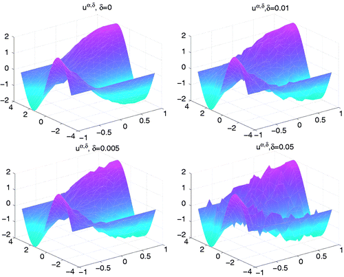
At last, we give the numerical results of the regularizing solution u^α,δ when α = α_H where C = 1 and γ = 1/2. In Figure 3, we give the exact solution u = Δf and the regularizing solutions u^α,δ for δ = 0.005, 0.01 and 0.05, respectively. The regularizing solutions u^α,δ can always approximate the exact solution u very well from Figure 3, which shows the validity and numerical stability of our scheme for computing the Laplacian operation. Notice that u|_∂Ω ≡ 0, the numerical results are still satisfactory near the boundary ∂Ω.

Figure 2. The relative errors RE of the regularizing solution u^α,δ for different noise level δ when α = α_H, α_G and α_M, respectively (left), the RE for α = α_G and different δ when q = 1, 0.6, 0.2 and 0, respectively (right).

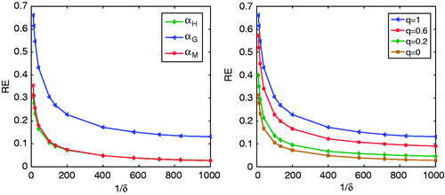
Figure 3. Exact solution u = Δf and the regularizing solutions u^α,δ for δ = 0.005, 0.01 and 0.05 when α = α_H.

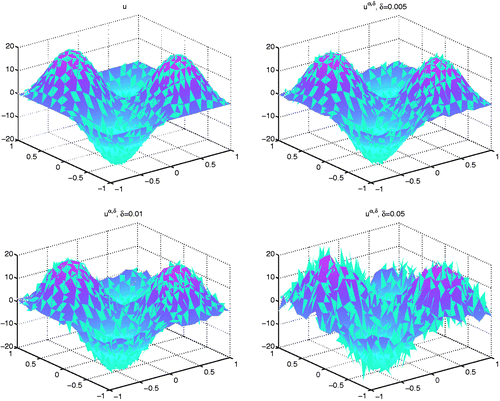
Table 1. The values of α*, α_H and the iteration number it for solving the generalized discrepancy principle.

δ	0.001	0.005	0.01	0.05	0.1
α*	1.659 × 10^−3	3.139 × 10^−3	4.495 × 10^−3	1.106 × 10^−2	1.692 × 10^−2
αH	1.659 × 10^−3	3.139 × 10^−3	4.495 × 10^−3	1.106 × 10^−2	1.692 × 10^−2
it	5	6	6	8	10

Table 2. The values of α_H, α_M, α_G and the relative errors RE of the corresponding regularizing solution u^α,δ.

δ	0.001	0.005	0.01	0.05	0.1
αH	1.674 × 10^−3	3.130 × 10^−3	4.513 × 10^−3	1.109 × 10^−2	1.667 × 10^−2
RE	2.792%	7.259%	10.57%	23.21%	31.41%
αG	7.814 × 10^−3	1.501 × 10^−2	2.223 × 10^−2	6.104 × 10^−2	9.883 × 10^−2
RE	13.12%	22.75%	30.44%	54.71%	66.13%
αM	1.583 × 10^−3	2.427 × 10^−3	3.300 × 10^−3	7.248 × 10^−3	1.034 × 10^−2
RE	2.670%	7.471%	11.17%	25.64%	35.50%

Example 2

Consider a function with non-zero boundary value given by then, it has

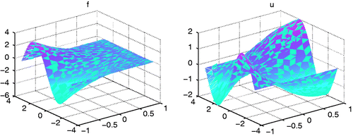
The functions f and its exact Laplacian operation u = Δ f are shown in Figure 4. Since f |_∂Ω ≢ 0, the functional transformation (2.1) should be done in advance. The noisy data f^δ is generated as the same way in Example 1. From the analysis in Section 2 we know the regularizing solution u^α,δ is satisfactory only in the interior part of Ω, hence, we assume the exact solution u is known on the point x ∈ Ω where its distance to ∂Ω is less than 0.2. For given noisy data f^δ, the regularizing solution u^α,δ is obtained by solving the boundary value problem (2.6)–(2.8), where the regularization parameter α is chosen by the generalized discrepancy principle with C = 1, γ = 1/2 using the iterative algorithm in the last section. The regularizing solutions u^α,δ for different noise level δ are shown in Figure 5. We can see that the regularizing solution is very nice for the exact data f. For different noise level δ, the regularizing solutions are still satisfactory in the interior part of Ω, when the exact solution u is specified near ∂Ω in advance.

Figure 4. The functions f and u = Δf.

Figure 5. The regularizing solutions u^α,δ for different noise level δ.

6. Application

In the section, we will show the application of our scheme for computing the Laplacian operation in the harmonic B_z algorithm of MREIT. The general idea of MREIT is to detect the conductivity distribution of a 3-dimensional biological tissue at each 2-dimensional slice from the information about internal electrical current. By injecting an electrical current between a pair of electrodes attached on the tissue surface, the information of the internal electrical current can be captured by using MRI scanner indirectly, with the measurement data of the magnetic flux density B_z along the main magnetic field direction. For more technical background, the readers are referred to 13,14 and the references therein. The simplification of this physical problem at a 2-dimensional slice can be described as follows.

Consider the mixed boundary value problem (24) where is the 2-dimensional slice of Ω, I is the input electrical current injected between a pair of electrodes , and u is the internal voltage induced by I. The z-component of the internal magnetic flux density induced by I is denoted as B_z, which can be represented as (25) in from the Ampere's law. The MREIT problem is to reconstruct the conductivity distribution σ in from the measurement data of B_z(x, y). Utilizing two suitable pairs of electrodes attached on with input electrical currents I_j, respectively, it had been proven that σ can be determined uniquely from the corresponding magnetic flux , see 35.

The harmonic B_z algorithm for MREIT problem constructs an approximation sequence from (26) where and (27) with u_j solves (6.1) for input electrical current I_j, j = 1, 2 through surface electrodes . As we can see, the data are applied in the iterative algorithm, whereas, the practical measurement data are . Hence, when the measurement data are contaminated, the stable computation of from the noisy data of is the key ingredient for the convergence of this iteration algorithm. By applying our scheme to compute the Laplacian from noisy measurement data, a numerical simulation problem is given as follows.

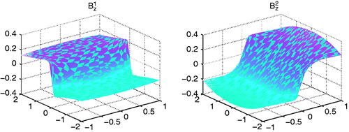
Consider a 2-dimensional domain with two pairs of electrodes The injected electrical currents through are I₁ = I₂ = 1, and the exact conductivity σ is simulated by where the function f(x, y) represents the grey level of the picture shown in Figure 6. Its value varied in [0, 255], where f(x, y) = 0 and f(x, y) = 255 indicate the black and white colour, respectively. The exact magnetic flux is simulated by (6.2) in our numerical simulation (Figure 7) and its noisy data are generated by where rand is a random number in (−0.5, 0.5).

Figure 6. The picture with grey level f.

Figure 7. The exact magnetic flux and .

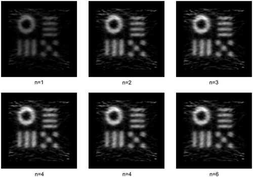
When applying our scheme to compute from the noisy data , we assume that the true conductivity σ* = 1 is known in . This assumption is needed for the convergence of the harmonic B_z algorithm 13, which just overcomes the defect of our scheme for computing the Laplacian operation near the boundary . Taking an arbitrary initial guess the relative errors of the inversion iterative sequence {σⁿ} are shown in Table 3 for different iteration number n and noise level δ. It can be concluded that the inversion results are satisfactory under reasonable noise level δ, due to the efficient scheme for computing ΔB_z from its noisy data. When δ = 3%, the inversion results of the conductivity for different iteration number n are given in Figure 8, showing the edges of true conductivity clearly.

Figure 8. The reconstructive results of σⁿ when noise level δ = 3%.

Table 3. The relative error E(n) of the iterative sequence σⁿ for different noise level δ and iteration number n.

	n = 0	n = 1	n = 2	n = 3	n = 4	n = 5	n = 6	n = 7
δ = 0%	0.4603	0.1469	0.0688	0.0547	0.0520	0.0514	0.0513	0.0513
δ = 1%	0.4603	0.1566	0.0991	0.0924	0.0916	0.0915	0.0914	0.0914
δ = 3%	0.4603	0.1801	0.1383	0.1334	0.1328	0.1327	0.1327	0.1327
δ = 5%	0.4603	0.1943	0.1621	0.1574	0.1566	0.1564	0.1564	0.1564

Acknowledgements

This work is supported by NSFC (No.10911140265).

References

- Cullum, J, 1971. Numerical differentiation and regularization, SIAM J. Num. Anal. 8 (1971), pp. 254–265.
- Ramm, AG, 1968. On numerical differentiation, Izv. Vyssh. Uchebn. Zaved. Mat. 11 (1968), pp. 131–134.
- Hanke, M, and Scherzer, O, 2001. Inverse problems light: Numerical differentiation, Am. Math. Monthly 108 (2001), pp. 512–521.
- Murio, DA, Mejia, CE, and Zhan, S, 1998. Discrete mollification and automatic numerical differentiation, Comput. Math. Appl. 35 (1998), pp. 1–6.
- Qu, R, 1996. A new approach to numerical differentiation and regularization, Math. Comput. Model. 24 (1996), pp. 55–68.
- Ramm, AG, and Smirnova, AB, 2001. On stable numerical differentiation, Math. Comput. 70 (2001), pp. 1131–1153.
- Wang, YB, Jia, XZ, and Cheng, J, 2002. A numerical differentiation method and its application to reconstruction of discontinuity, Inv. Probl. 18 (2002), pp. 1461–1476.
- Egger, H, and Engl, HW, 2005. Tikhonov regularization applied to the inverse problem of option pricing: Convergence analysis and rates, Inv. Probl. 21 (2005), pp. 1027–1045.
- Hein, T, and Hofmann, B, 2003. On the nature of ill-posedness of an inverse problem arising in option pricing, Inv. Probl. 19 (2003), pp. 1319–1338.
- Johnson, RP, 1990. Contrast based edge detection, Pattern Recog. 23 (1990), pp. 311–318.
- Wan, XQ, Wang, YB, and Yamamoto, M, 2006. Detection of irregular points by regularization in numerical differentiation and application to edge detection, Inv. Probl. 22 (2006), pp. 1089–1103.
- Lamm, PK, 2000. "A Survey of Regularization Methods for First-Kind Volterra Equations". In: Surveys on Solution Methods for Inverse Problems. Vienna: Springer-Verlag; 2000.
- Liu, JJ, Seo, JK, Sini, M, and Woo, EJ, 2007. On the convergence of the harmonic Bz algorithm in magnetic resonance electrical impedance tomography, SIAM J. Appl. Math. 67 (2007), pp. 1259–1282.
- Liu, JJ, Seo, JK, and Woo, EJ, 2011. A posteriori error estimate and convergence analysis for conductivity image reconstruction in MREIT, SIAM J. Appl. Math. 70 (2011), pp. 2883–2903.
- Ahn, S, Choi, UJ, and Ramm, AG, 2006. A scheme for stable numerical differentiation, J. Comput. Appl. Math. 186 (2006), pp. 325–334.
- Nakamura, G, Wang, SZ, and Wang, YB, 2008. Numerical differentiation for the second order derivatives of functions of two variables, J. Comput. Appl. Math. 212 (2008), pp. 341–358.
- Wang, YB, Hon, YC, and Cheng, J, 2006. Reconstruction of high-order derivatives from input data, J. Inv. Ill-Posed Probl. 14 (2006), pp. 205–218.
- Wang, YB, and Wei, T, 2005. Numerical differentiation for two-dimensional scattered data, J. Math. Anal. Appl. 312 (2005), pp. 121–137.
- Xu, HL, and Liu, JJ, 2011. Stable numerical differentiation for the second order derivatives, Adv. Comput. Math. 33 (2011), pp. 431–447.
- Engl, HW, Hanke, M, and Neubauer, A, 1996. Regularization of Inverse Problems. Dordrecht: Kluwer; 1996.
- George, S, and Nair, MT, 1993. An a posteriori parameter choice for simplified regularization of ill-posed problems, Integr. Equat. Oper. Theory 16 (1993), pp. 392–399.
- George, S, and Nair, MT, 1994. A class of discrepancy principles for simplified regularization of ill-posed problems, J. Austral. Math. Soc., Ser. B 36 (1994), pp. 242–248.
- Groetsch, CW, and Guacaneme, J, 1987. Arcangeli's method for Fredholm integral equations of the first kind, Proc. Am. Math. Soc. 99 (1987), pp. 256–260.
- Schock, E, 1984. On the asymptotic order of accuracy of Tikhonov regularization, J. Optim. Theory Appl. 44 (1984), pp. 95–104.
- Tautenhahn, U, 2002. On the method of Lavrentiev regularization for nonlinear ill-posed problems, Inv. Probl. 18 (2002), pp. 191–207.
- Guacaneme, JE, 1988. On simplified Tikhonov regularization, J. Optim. Theory Appl. 58 (1988), pp. 133–138.
- Hamarik, U, Raus, T, and Palm, R, 2008. On the analog of the monotone error rule for parameter choice in the (iterated) Lavrentiev regularization, Comput. Meth. Appl. Math. 8 (2008), pp. 237–252.
- Hamarik, U, and Raus, T, 2009. About the balancing principle for choice of the regularization parameter, Num. Funct. Anal. Optim. 30 (2009), pp. 951–970.
- Nair, MT, and Schock, E, 2003. On the Ritz-method and its generalization for ill-posed equations with non-self adjoint operators, Int. J. Pure Appl. Math. 5 (2003), pp. 119–134.
- Nair, MT, and Tautenhahn, U, 2004. Lavrentiev regularization for linear ill-posed problems under general source conditions, Z. Anal. Anwendung. 23 (2004), pp. 167–185.
- Hoang, NS, and Ramm, AG, 2009. A discrepancy principle for equations with monotone continuous operators, Nonlinear Anal. 70 (2009), pp. 4307–4315.
- Kunisch, K, and Zou, J, 1998. Iterative choices of regularization parameters in linear inverse problems, Inv. Probl. 14 (1998), pp. 1247–1264.
- Liu, JJ, and Ni, M, 2008. A model function method for determining the regularization parameter in potential approach for the recovery of scattered wave, Appl. Num. Math. 58 (2008), pp. 1113–1128.
- Wang, ZW, and Liu, JJ, 2009. New model function methods for determining regularization parameters in linear inverse problems, Appl. Num. Math. 59 (2009), pp. 2489–2506.
- Kwon, O, Pyo, HC, Seo, JK, and Woo, EJ, 2006. Mathematical framework for Bz-based MREIT model in electrical impedance imaging, Comput. Math. Appl. 51 (2006), pp. 817–828.