Space-variable thermophysical properties identification in nanocomposites via integral transforms, Bayesian inference and infrared thermography

Abstract

Simultaneous estimation of space-variable thermal conductivity and heat capacity in heterogeneous samples of nanocomposites is dealt with by employing a combination of the generalized integral transform technique (GITT), for the direct problem solution, Bayesian inference as implemented with the Markov chain Monte Carlo (MCMC) method, for the inverse analysis and infrared thermography, for the temperature measurements. Another aspect of the proposed approach is the integral transformation of the thermographic experimental data along the space variable, which allows for a significant data compression since the inverse analysis is undertaken within the transformed field. Results are presented for the covalidation of the experiment with a homogeneous polyester plate, as well as for a plate made of polyester–alumina nanoparticles composite with abrupt variation of the filler concentration.

Keywords:

• heterogeneous media
• nanocomposites
• Bayesian inference
• integral transforms
• infrared thermography

Nomenclature

	=	parameters in parametrized transient behaviour of the heat flux, Equations (10a–c)
	=	parametrized transient behaviour function of the applied heat flux, Equations (10a–c)
cp(x)	=	specific heat
d(x)	=	linear dissipation operator coefficient
	=	transformed source terms, Equation (4c)
heff(x)	=	effective heat transfer coefficient
	=	parameters in the heat transfer coefficient filtering function, Equation (11)
k(x)	=	thermal conductivity
	=	parameters in the thermal conductivity filtering function
Lx	=	plate length
Lz	=	plate thickness
N	=	truncation order in temperature expansion
Nw, Nk, Nd	=	truncation orders for the expansions of the coefficients w(x), k(x) and d(x)
NP	=	number of parameters to be estimated
Ni	=	normalization integrals in eigenvalue problem, Equations (4a, b)
	=	number of states of the burn-in period in the MCMC method
	=	number of parameters appearing in the filtering functions for , and , respectively
	=	probability density
P(x, t)	=	source term
q(x, t)	=	applied heat flux
qw(x)	=	applied heat flux spatial distribution
	=	parameters in the applied heat flux spatial variation, Equations (10a–c)
t	=	time variable
Tm(x, t)	=	temperature distribution
	=	temperature of surrounding air
	=	experimental temperature measurements
w(x)	=	thermal capacity
	=	parameters in the thermal capacity filtering function
x	=	space coordinate
	=	end position of the electrical resistance over the plate
	=	transition point in the step function , Equation (13c)
Y	=	vector of measurements
P	=	vector of unknown parameters

	=	acceptance factor in the Metropolis–Hastings algorithm, Equation (7a)
	=	eigenfunctions of the variable equation coefficients expansions
	=	parameter that controls the transition sharpness in , Equation (13c)
	=	step function, Equation (13c)
	=	candidategenerating density
μ	=	eigenvalues of the direct problem
ψ	=	eigenfunctions of the direct problem
ρ(x)	=	space-variable density

i, j	=	order of eigenquantities
_	=	integral transform
∼	=	normalized eigenfunction
f	=	filtering function in coefficients expansion

1. Introduction

Heat conduction problems defined in heterogeneous media involve space variations of the physical properties in different forms, depending on the type of heterogeneity that prevails, such as large-scale variations in functionally graded materials, abrupt variations in laminated media and random variations due to fluctuations of local concentrations in dispersed systems 1–5. The accurate determination of local variations in physical properties within heterogeneous media requires an experimental technique that provides abundant information on spatially distributed measurements, in order to provide a firm basis for application of the appropriate inverse problem analysis. In addition, as the morphology of the medium directly influences the spatial behaviour of the physical properties, it becomes critical not to disturb the structure along the experimental campaign by introducing intrusive sensors, such as thermocouples in the case of temperature measurements. Therefore, aiming at the identification of spatially variable thermophysical properties, the adoption of the non-intrusive technique of infrared thermography becomes of major interest, providing a large volume of measurements, both in space and time, and offering new perspectives towards the analysis of heat conduction in heterogeneous media 6–8. On the other hand, the large volume of measurements provided by the infrared thermography technique yields an additional challenge for the inverse analysis, in terms of processing such a large amount of information. Thus, the development of techniques that are able to handle the large amount of temperature measurements provided by infrared thermography within feasible computation time becomes of major interest 9,10.

This work thus provides an experimental demonstration of a recently proposed inverse analysis methodology 10,11 that combines the integral transform method for the direct problem solution and for the compression of the experimental data, which is obtained by infrared thermography, as well as Bayesian inference for the inverse problem solution. Bayesian inference has been demonstrated to be a powerful tool in the estimation of spatially variable equation and boundary condition coefficients in heat diffusion problems 10–12, by employing the Markov chain Monte Carlo (MCMC) method, with the Metropolis–Hastings algorithm for the sampling procedure 13–16. This sampling procedure used to recover the posterior distribution is in general the most expensive computational task, since the direct problem is calculated for each state of the Markov chain. In this context, the use of a fast, accurate and robust computational implementation of the direct solution is extremely important. Thus, the integral transformation method 17–22 becomes very attractive for the combined use with the MCMC method. Such is the case because analytical expressions can be obtained for different quantities required in the implementation, thus avoiding repetitive numerical tasks 22. Also, instead of seeking the function estimation in the form of a sequence of local values for the variable coefficients, an alternative path is utilized based on the eigenfunction expansion of the coefficients to be estimated 22. Another important aspect of this combined methodology is the analysis of the inverse problem in the transformed temperature field, instead of employing the directly measured temperature data along the domain. Thus, the experimental spatially distributed temperature values at each time are first integral transformed to yield transformed temperature values of increasing order. This procedure is particularly advantageous when a substantial amount of experimental measurements are available, such as with the infrared thermography technique employed here, permitting a remarkable data compression.

In order to demonstrate the applicability of the proposed thermophysical properties estimation approach, an experiment was built and tested 23,24, which employs samples made of thin plates partially heated with an electrical resistance on one surface, while the other surface is exposed to the infrared thermography system. Studies have been undertaken with this methodology, demonstrating the recovery of the homogeneous thermophysical properties of a bakelite plate without the assumption or previous knowledge of its uniform distribution behaviour 24. In another verification, we have used polystyrene plates manufactured with a controlled thickness that varies linearly along the plate's length, modelling the variable thickness as space-varying effective thermophysical properties 25, which have then been estimated.

In this article, the proposed combined approach is further challenged, as applied to identify the thermophysical properties of an actual heterogeneous material. Controlled experiments are performed with a thin nanocomposite plate, made of polyester resin and alumina nanoparticles, with an abrupt variation in the thermophysical properties as a consequence of the variation in the filler concentration. Furthermore, two other novel aspects of the present inverse analysis are investigated. First, we compare the use of informative and non-informative filtering functions in the properties eigenfunction expansions. Second, the effects of the heater position on the estimation procedure are examined, showing that significant improvements can be achieved by properly locating the heater across the region of spatial variation on the properties to be estimated.

2. Direct problem solution

We consider a one-dimensional special case of the general formulation on transient heat conduction presented in 22, for the transversally averaged temperature field within a thermally thin plate, in the region x  [0, L_x]. The formulation includes the space-variable thermal conductivity and heat capacity, as shown in problem (1). The equation coefficients , and are thus responsible for the information related to the heterogeneity of the medium. The heat conduction equation with initial and boundary conditions is given by (1) (2) (3) where

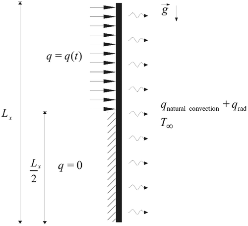
Problem (1) models a typical one-dimensional transient thermal conductivity experimental setup for a thermally thin plate, including prescribed heat flux at one surface and convective and radiative heat losses at the opposite surface (Figure 1), and based on a lumped formulation across the sample thickness. The exposed surface allows for temperature measurements acquisition via infrared thermography 23–25.

Figure 1. Schematic representation of the experimental setup for thermophysical properties identification in heterogeneous media.

The formal exact solution of problem (1) is then obtained with the classical integral transform method 22, and is written as (4) where the eigenvalues and eigenfunctions are obtained from the eigenvalue problem that contains the information about the heterogeneous medium in the form: (5) with boundary conditions (6)

Also, the other quantities that appear in the exact solution (2) are computed after solving problem (3), such as (7) (8) (9)

The generalized integral transform technique (GITT) is employed here for the solution of the Sturm–Liouville problem (Equations 3a–c) via the proposition of a simpler auxiliary eigenvalue problem, and expanding the unknown eigenfunctions in terms of the chosen basis. Also, the variable equation coefficients are themselves expanded in terms of known eigenfunctions, so as to allow for a fully analytical implementation of the coefficients matrices in the transformed system. For instance, the coefficients , k(x) and d(x) are expanded in terms of eigenfunctions, together with filtering solutions (identified by the subscript f), in the following form: (10) (11) (12) (13) (14) (15) where is the weighting function for the chosen normalized eigenfunction . The expansion basis may be chosen by employing the same auxiliary problem, but with first-order boundary conditions, while the filtering function could be a simple analytic function that satisfies the boundary values for the original coefficients or just an average value of the respective coefficient. The filtering functions are used to incorporate as much information as possible regarding the functional form of each space-variable coefficient, in order to enhance the convergence of the eigenfunction expansions. As a consequence, the number of expansion coefficients to be estimated through the inverse analysis can be reduced.

3. Inverse problem solution

In the Bayesian approach, inference is drawn by constructing the joint probability distribution of all unobserved quantities, based on all that is known about them. This knowledge incorporates previous information about the phenomena under study and is also based on values of observed quantities when they are available. This approach is based on Bayes’ theorem, which can be written as 13,15 (16)

In summary, solving an inverse problem within the Bayesian framework may be broken into three subtasks: (i) based on all information available for the unknown , find a prior probability density that reflects judiciously this prior information; (ii) find the likelihood function that describes the interrelation between the observations and the unknowns and (iii) develop methods to explore the posterior probability density .

When it is not possible to analytically obtain the corresponding posterior distributions, one needs to use a method based on simulation. The inference based on simulation techniques uses samples from the posterior to extract information about it. Several sampling strategies are proposed in the literature, including the Monte Carlo method via Markov chain (MCMC), adopted in this work.

The most commonly used MCMC sampling algorithm is the Metropolis–Hastings employed here 13,15. The Metropolis–Hastings algorithm uses the same idea of the rejection methods, i.e. a value is generated from an auxiliary distribution and accepted with a given probability. This correction mechanism ensures the convergence of the chain to the equilibrium distribution. The following steps briefly summarize the Metropolis–Hastings algorithm employed for the construction of the chains:

Step 1

Sample a candidate from the candidate-generating density .

Step 2

Calculate (17)

Step 3

If , then (18) else, (19) where is a random number from an uniform distribution between 0 and 1.

Step 4

Return to Step 1 in order to generate the chain .

We should stress that the first states of this chain must be discarded until the convergence of the chain is reached. These ignored samples are called the burn-in period, whose length will be denoted by .

In this work, as the candidate-generating density we have used normal distributions centred in the current state. In this case, is symmetric, i.e. the probability to move from to is the same as to move from to , so . Thus, Step 2 is simplified and Equation (7a) can be rewritten as (20)

The unknown quantities in this work, the variable thermal properties and the effective heat transfer coefficient, were expressed as eigenfunction expansions, which significantly reduces the number of parameters to be estimated. The truncation orders and the choices of filtering functions in the proposed expansions, Equations (5a–f), govern the number of parameters to be estimated. Thus, the total number of parameters is given by the sum of parameters in each expansion, including the number of parameters in each filter function, and the number of parameters in the heat flux expression, which are also to be estimated. Therefore, we have: (21) where N_kF, N_wF and N_dF are the number of parameters appearing in the filter functions for k(x), w(x) and d(x), respectively.

Another important aspect of this study is the solution of the inverse problem in the transformed field, from the integral transformation of the experimental temperature data, thus compressing the experimental measurements in the space variables into a few transformed temperature modes. Once the experimental spatially distributed temperature readings have been obtained, one proceeds to the integral transformation of the temperature field at each time through the integral transform pair below: (22) (23)

Both the direct and inverse problem solutions were implemented in the symbolic–numerical computation platform Mathematica 26.

4. Experimental setup and procedure

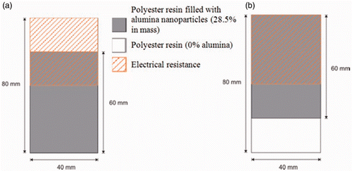
The experimental setup presented in Figure 2 employs temperature measurements obtained from the infrared camera FLIR SC660, a high performance infrared system with 640 × 480 image resolution and a temperature range of −40°C to 1500°C. The main components of the setup are marked in Figure 2 as: (a) IR camera (FLIR SC660); (b) camera stand for vertical experiment configuration; (c) frame with sandwiched heated plates; (d) sample support; (e) data acquisition system (Agilent 34970-A) and (f) microcomputer for data acquisition. Figure 3 shows the nanocomposite plate used in this experiment, which is composed by polyester resin as matrix and alumina nanoparticles as filler, manufactured in such a way that ¾ of the plate's length has 28.5% of alumina nanoparticles in mass and the other ¼ of the plate's length is composed only by polyester resin, with no addition of filler. The thickness of the plate is 1.51 mm and its lateral and vertical dimensions are 40 × 80 mm. An electrical resistance (38.2 Ω) was employed for the heating of the plate, with the same lateral dimensions as of the plate but half the length (40 × 40 mm), joined here at the upper half of the plate's height with the aid of a thermal compound paste. As a reference case, we have used a pair of homogeneous polyester resin plates in a plate–heater–plate sandwich setup; this case is hereafter called Case 1. For the nanocomposite plate we have set up a plate–heater–insulation sandwich setup and investigated two cases by varying the position of the plate with respect to the electrical resistance: first, the portion with no addition of filler has been placed in contact with the electrical resistance and for the last case the plate has been turned upside down. These experimental setups are hereafter called Cases 2 and 3, respectively, and are schematically represented in Figure 4. In order to reduce uncertainty in the IR camera readings, the plate surface that faces the infrared camera was painted with a graphite ink, which brought its emissivity to , as stated by the ink manufacturer.

Figure 2. General view of the experimental setup for the infrared thermography analysis.

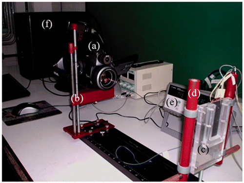
Figure 3. Polyester resin–alumina nanocomposite plate used in the experiment with dimensions 1.51 mm (thickness), 40 mm (width) and 80 mm (length).

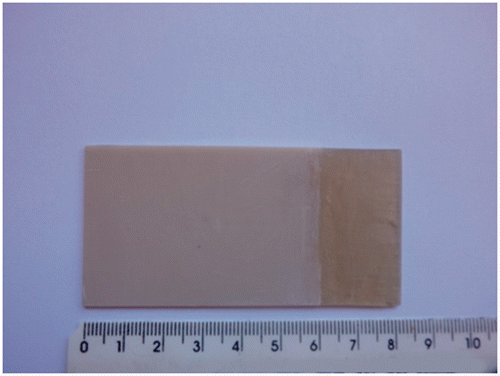
Figure 4. Schematic representation of the experimental setup involving the nanocomposite sample for (a) Case 2 and (b) Case 3.

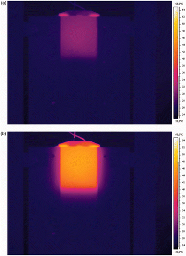
The experimental procedure is initiated by prescribing a voltage difference to be imposed on the electrical resistance, with a DC voltage regulator. The data acquisition is started and, after preliminary measurements used to allow for averaging the initial conditions, the DC source is turned on to heat the sample plates (a nominal voltage of 8 V has been applied through the DC source in all experiments). The temperature increase may be followed through computer monitoring. For instance, Figure 5 illustrates the images produced by the FLIR SC660 camera acquisition system, both 40 s after that the DC source is turned on, in Figure 5(a), and after 300 s, when the heated plate image is much brighter, in Figure 5(b). Once steady state is achieved, the DC source is turned off.

Figure 5. Infrared camera image acquired at (a) 40 s after the DC source is turned on and (b) t = 300 s, during heating period.

5. Results and discussion

Some verifications have been performed in order to test the constructed setup. First, we have observed a practically perfect superposition of the temperature measurements by thermocouples (type K) installed at a bakelite plate sample, with the infrared camera measurements. Then, the temperature measurements from three independent experimental runs have demonstrated the repeatability of the experimental procedure, which resulted on an average standard deviation of 0.11°C 25.

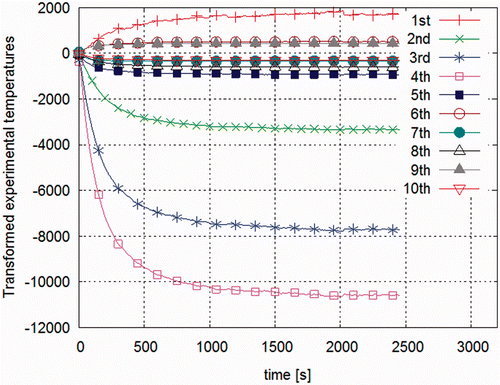
The number of pixels of the infrared camera in the vertical direction provides 325 spatial measurements along the 80 mm plate and, with the frequency of measurements used, 222 transient measurements per pixel are available. Figure 6 illustrates the time evolution of the transformed temperature modes, consecutively numbered up to the 10th transformed potential, as obtained from Equation (9a). The transformed temperatures are in fact the quantities that are employed in the inverse problem analysis. Although the first four transformed potentials of the measurements are significantly more important than the subsequent ones, for the results presented below we preferred to use for the inverse analysis the first ten transformed potentials. Indeed, the determinant of the information matrix does not increase substantially, and hence the conditioning of the inverse problem, if the number of transformed modes is increased beyond, as examined in ref. 10 by using simulated data. Therefore, a significant data compression of more than 96% is achieved, as one chooses to solve the inverse problem in the transformed temperature domain. In fact, we drop from a total of 72,150 temperature measurements to only 2220 data points in the transformed domain.

Figure 6. Time evolution of the first ten integral transformed experimental temperatures.

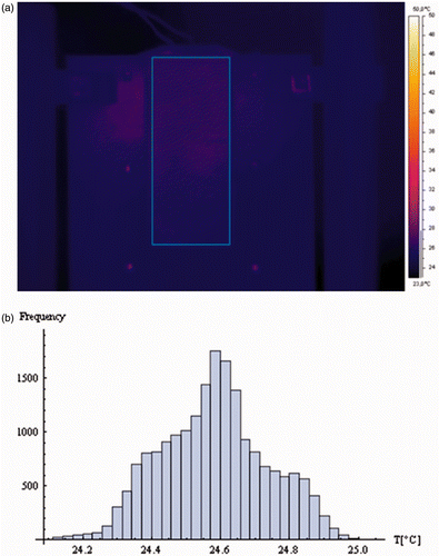
For the inverse analysis, the hypothesis of a Gaussian likelihood has been adopted. Figures 7 and 8 show the infrared images of plates with uniform temperatures, as well as the histogram of the measurements of the camera pixels. These histograms clearly show that the measurement errors can be fairly well approximated by a Gaussian distribution. We point out that a quite low acquisition frequency has been used (0.1 frame per second), which avoids autocorrelation of the measurements and significantly minimizes the noise due to time increments 27. Besides that, the temperature measurements obtained with the infrared camera were directly used for the inverse analysis, without any spatial averaging or filtering, which could make the measurements correlated. Further discussions on the local noise level of uncooled microbolometric infrared cameras are found in ref. 27.

Figure 7. (a) Thermal image of a 4 × 4 cm uniformly heated plate and (b) histogram of the temperature measurements of the uniformly heated plate.

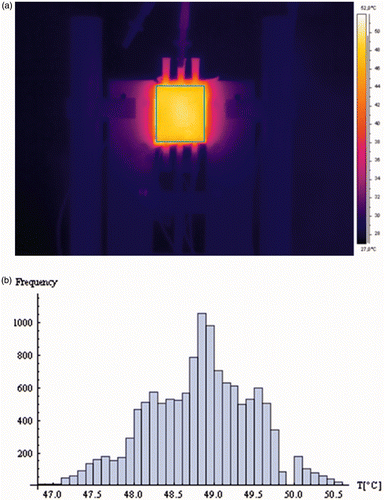
Figure 8. (a) Thermal image of the 8 × 4 cm plate experiment setup employed in this work. The plate is in its initial condition (before turning the heater on) and (b) histogram of the temperature measurements of the plate.

The time variation of the applied heat flux, which accounts for the thermal capacity of the resistance itself and of the thermal paste, besides the thermal contact resistance, has been parametrized. The applied heat flux is considered here to be given by where gives the length of the electric resistance over the plate. Therefore, the unheated portion of the plate corresponds to a heat flux . Since the dissipated power in the resistance is accurately measured, Equation (1a) is thus divided by , and then the estimated parameters can be obtained by multiplying each one by the measured heat flux value and its associated uncertainty.

The effective heat transfer coefficient, d(x), has been expanded in eigenfunctions, such as given by Equations (5e, f). In light of the nature of the applied heating, a filter was considered in the form of a step function that assumes two different characteristic values for the heat transfer coefficient at the heated and unheated plate portions, that is, (24)

The initial guesses for h₁ and h₂ were then obtained from correlations for natural convection over vertical plates and linearization of the radiative heat flux.

As previously discussed, the truncation orders of the expansions for each unknown parameter govern the number of parameters in the estimation procedure. The total number of parameters refers to the filters and expansions for the thermal conductivity, heat capacity and effective heat transfer coefficient, in addition to the parameters , and in Equations (10a–c), that control the time variation of the applied heat flux, so that we have: (25)

In order to have available reference values for the thermophysical properties of the polyester resin employed in this study, we have performed the inverse analysis of Case 1 with the homogeneous pure polyester resin sample. In this case, we have adopted normal priors with 15% standard deviation, centred in the literature values 28, obtaining the estimates: °C⁻¹ and °C⁻¹, for the thermal conductivity and heat capacity, respectively.

We now consider for the inverse analysis the estimation of the space-varying properties of the nanocomposite plate with the setup of Case 2 (Figure 4a). We assume the filter for the thermal conductivity and heat capacity in the form of linear functions that vary between the end values and , and and , respectively. For these parameters we have adopted normal priors, with 15% standard deviation, centred in the literature values for the polyester resin 28 and in Lewis–Nielsen's formula prediction 29 for the region filled with alumina nanoparticles. For the results presented below, seven terms are used for the expansions in Equations (5a–d) of w(x) and k(x), while three terms are used in the expansion of d(x). The inverse analysis with simulated data of refs 10–12 reveals that accurate estimates can be obtained for the unknown parameters, with such parametrization. In fact, the maximum magnitude of the determinant of the information matrix rapidly decreases by increasing the number of unknown parameters in the expansions used for w(x), k(x) and d(x), as a result of the ill-posed character of the inverse problem. Table 1 presents the parameters and type of prior information that has been adopted in this inverse analysis (N = Gaussian distribution, U = non-informative uniform distribution) as well as the estimated mean values obtained for each one of the parameters. Markov chains of states were used, and the statistics were computed by neglecting the first states needed for the warm up of the chains. 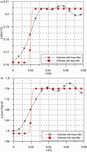For the sake of illustration, Figure 9(a) and (b) shows, respectively, the evolution of the Markov chains for the parameter and for the first coefficient in the expansion of the thermal conductivity in Equations (5c, d), , where one can clearly observe the convergence of the states. Figure 10(a) and (b) presents, respectively, the estimated spatial variations for the thermal conductivity and heat capacity, with their 99% confidence intervals, as well as the initial guess employed in this test case. One must observe that with the linear filter functions used for the thermophysical properties in this case, which does not provide informative priors regarding their functional forms, the proposed methodology was able to identify a transition of the space-varying properties from the end values at towards constant values. Figure 10(a) and (b) shows that this transition is centred around , where, in fact, a sharp interface exists between the two materials that compose the plate. Figure 11(a) depicts the residuals between calculated and experimental quantities for the first five transformed temperature modes. Although presenting some correlation, which results from the integral transformation procedure that is truncated at the low order of 10 modes, the residuals are small. Similar behaviour can be observed for the residuals in the temperature field, presented in Figure 11(b) at three different positions. Some tests have been performed with more than seven terms in the expansions of the sought coefficients. However, as expected from the analysis of the determinant of the information matrix 10–12, no improvements were observed in the estimated quantities. This is due to the small sensitivity coefficients of the coefficients of higher order in the expansions.

Figure 9. (a) Markov chain evolution of the parameter in the linear filter in Equations (5c, d) and (b) Markov chain evolution of the first coefficient in the expansion in Equations (5c, d), , considering a linear filter.

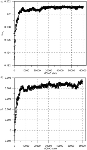
Figure 10. (a) Estimated thermal conductivity with linear filter and 99% confidence intervals and (b) estimated heat capacity with linear filter and 99% confidence intervals.

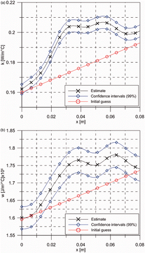
Figure 11. (a) Residuals (m°C) between calculated and experimental temperature modes in the transformed domain (linear filter case) and (b) residuals (°C) between calculated and experimental temperatures at three different positions (linear filter case).

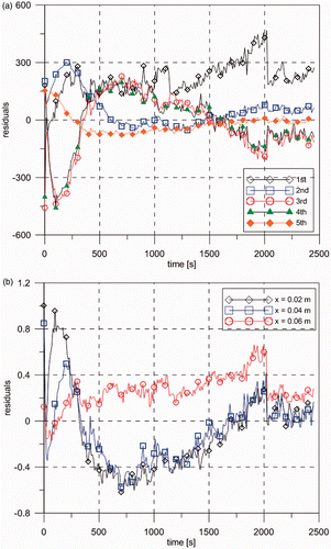
Table 1. Prior information and estimated parameters.

Parameter	Prior information	Estimates (mean values)
Thermal conductivity (Case 2 – linear filter)
(W m^−1°C^−1)	N (0.16, 15%)	0.1621
(W m^−1°C^−1)	N (0.193, 15%)	0.201
	U (−0.0279, 0.0279)	0.00427344
	U (−0.00698, 0.00698)	0.0002019
	U (−0.00931, 0.00931)	−0.0007205
	U (−0.00349, 0.00349)	−0.0003482
	U (−0.00559, 0.00559)	−0.0004592
	U (−0.00232, 0.00232)	0.0002434
	U (−0.00399, 0.00399)	0.0001065
Heat capacity (Case 2 – linear filter)
(J m^−3°C^−1)	N (1.595 × 10^6)	1.601 × 10^6
(J m^−3°C^−1)	N (1.736 × 10^6)	1.74 × 10^6
	U (−255921.0, 255921.0)	17048.43
	U (−63980.3, 63980.3)	−1479.72
	U (−85307.0, 85307.0)	−1193.36
	U (−31990.1, 31990.1)	−3341.41
	U (−51184.2, 51184.2)	−477.34
	U (−21326.8, 21326.8)	668.28
	U (−36560.2, 36560.2)	−1002.42
Heat transfer coefficient (Case 2 – linear filter)
(W m^−1°C^−1)	N (15.03, 5%)	14.286
(W m^−1°C^−1)	N (11.63, 5%)	12.041
	N (−0.23, 5%)	−0.2492
	N (0.69, 5%)	0.7197
	N (−0.044, 5%)	−0.0437
Applied heat flux (Case 2 – linear filter)
	N (0.19, 5%)	0.197
	N (0.00332, 5%)	0.00315
	N (0.66, 5%)	0.64

On the basis of the observations described above, we now consider a filter function for the thermophysical properties that approximates a step transition between the end values at x = 0 and x = L_x, in the form: (26) where (27)

In Equation (13c), is a parameter that controls the transition sharpness and is the transition point. Both are considered as fixed parameters, not to be estimated with the inverse analysis, the values of which are taken as γ = 1500 m⁻¹ and  = 0.02 m (based on the above observations with the linear filter function).

Figure 12(a) and (b) shows the estimated spatial variations for the thermal conductivity and heat capacity obtained with the experimental arrangement of Case 2 (see Figure 4a), but with the filter function given by Equations (13). The estimated 99% confidence intervals and the employed initial guesses are also presented in these figures. Similar to the case examined above with the linear filter functions, the values used for the end parameters were obtained from normal priors, with 15% standard deviation, centred in the literature values for the polyester resin 28 and in Lewis–Nielsen's formula prediction 29 for the region filled with alumina nanoparticles. Figure 13(a) depicts the residuals between calculated and experimental quantities for the first five transformed temperature modes, while Figure 13(b) presents the residuals in the temperature field at three measurement positions. A comparison of Figures 11 and 13 reveals that both estimates, with the linear filter and with the step function filter, yield similar correlated residuals patterns, because the inverse analysis is performed with a reduced number of modes in the transformed domain. Nevertheless, the magnitude of the residuals obtained with the step function filter case are smaller than those obtained with the linear filter function, especially when considering the transformed potentials which are in fact used in the inverse analysis (see Figures 11a and 13a). This clearly indicates the more accurate estimates obtained with the step filter function. A comparison of the estimates obtained via the linear filter and the step function filter is presented in Figure 14(a) and (b). These figures show that, even without an informative prior in the filter function, like the linear variation considered here, the proposed methodology was able to identify the transition that occurs due to the variation of filler concentration in the nanocomposite plate.

Figure 12. (a) Estimated thermal conductivity with the step function filter and (b) estimated heat capacity with the step function filter.

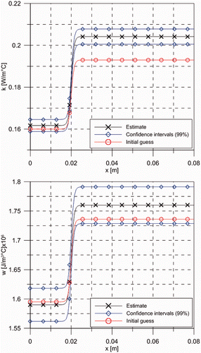
Figure 13. (a) Residuals (m°C) between calculated and experimental temperature modes in the transformed domain (step function filter case) and (b) residuals (°C) between calculated and experimental temperatures at three different positions (step function filter case).

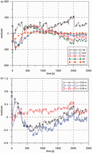
Figure 14. (a) Comparison of the mean values estimated for the thermal conductivity curves obtained with the linear filter and with the step function filter and (b) comparison of the mean values estimated for the heat capacity curves obtained with the linear filter and with the step function filter.

In order to provide a better assessment on the estimates obtained, we now compare the experimental arrangements of Cases 2 and 3 (see Figure 4). The approximate step filter function given by Equations (13) is used for this comparison, with γ = 1500 m⁻¹ and given by the transition point of materials in the manufactured plate. The remaining quantities, such as the number of expansion terms used in the eigenfunction approximations of Equations (5) and the prior distributions, were the same as specified above. Table 2 presents the estimated thermophysical properties obtained with the experimental arrangements of Cases 1–3, where states in the MCMC method have been generated, being the first states neglected in order to achieve the equilibrium of the chains. One may observe that the estimates obtained for the polyester resin properties of the nanocomposite plate in Case 2 are very close to those obtained in Case 1, where the experimental setup involved homogeneous polyester resin plates. On the other hand, the estimated parameters for the polyester in Case 3 are not in good agreement with those estimated for Case 1. That is probably because for Case 3 the portion of the nanocomposite plate composed with polyester resin without addition of filler has been placed away from the applied heat flux. This result was expected, since this homogeneous portion of the plate suffers a smaller variation of temperature during the experiment, yielding locally low sensitivity coefficients for the parameters. For the portion of the nanocomposite plate corresponding to the polyester resin filled with alumina nanoparticles, it may be observed that Cases 2 and 3 yield estimates very close to each other. The estimated values for the thermal conductivity are slightly higher than those provided by the Lewis–Nielsen formula 29, and similar results have been observed in ref. 30.

Table 2. Prior information and estimated thermophysical properties in Cases 1–3. A step filter has been used for Cases 1 and 2.

Property	Material	Prior	Estimates (mean values)
Case 1
(W m^−1°C^−1)	Polyester	N (0.16, 15%)	0.159
(J m^−3°C^−1)	Polyester	N (1.595 × 10^6, 15%)	1.566 × 10^6
Case 2
(W m^−1°C^−1)	Polyester	N (0.16, 15%)	0.162
	Polyester + alumina	N (0.193, 15%)	0.204
(J m^−3°C^−1)	Polyester	N (1.595 × 10^6, 15%)	1.59 × 10^6
	Polyester + alumina	N (1.736 × 10^6, 15%)	1.760 × 10^6
Case 3
(W m^−1°C^−1)	Polyester	N (0.16, 15%)	0.149
	Polyester + alumina	N (0.193, 15%)	0.203
(J m^−3C^−1)	Polyester	N (1.595 × 10^6, 15%)	1.529 × 10^6
	Polyester + alumina	N (1.736 × 10^6, 15%)	1.743 × 10^6

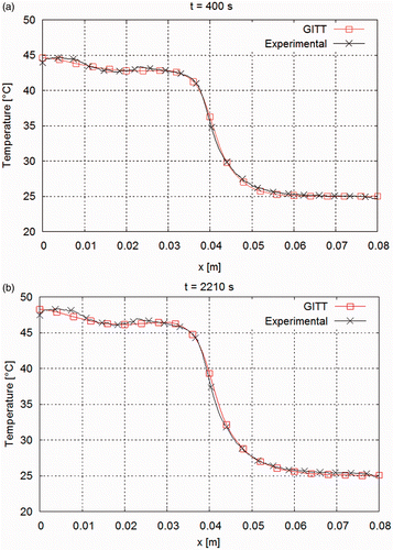
Figure 15 presents the estimated heat transfer coefficient for Cases 1–3. One may observe that the three curves show similar behaviour, especially for Cases 2 and 3, where the estimated curves are very near each other – we stress that Cases 2 and 3 employed the same plate sample, but with different positions of the material sharp transition with respect to the heater. Although, the heat transfer coefficient in this experiment is also function of temperature, because of free convection and radiation, the obtained results show that such non-linear effects are not significant for the cases examined. In fact, in order to further illustrate the accuracy of the proposed approach for the identification of the spatially varying thermophysical properties, we present a comparison of experimental temperature measurements and predictions obtained with the utilization of the estimated parameters in an independent computer program developed by our group for the direct problem solution 31. The measurements and the simulations refer to Case 2 and the parameters used in the simulation were those estimated with the linear filter function. Figure 16(a) and (b) presents the experimental and theoretically predicted time evolutions of the temperatures at and , respectively, up to steady state, whereas Figure 17(a) and (b) shows the vertical spatial distribution of the temperatures at times t = 400 s and t = 2210 s, respectively. An excellent agreement is observed in Figures 16 and 17, between the experimental data and the temperatures predicted with our independent direct problem solution, by using the parameters estimated with the present inverse analysis.

Figure 15. Estimated heat transfer coefficient, , in Cases 1–3.

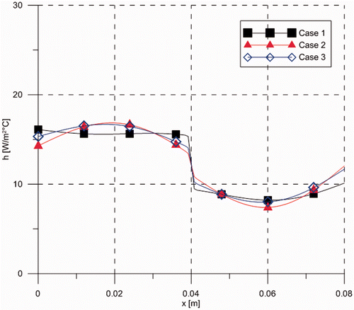
Figure 16. (a) Time evolution of the temperature at x = 0.02 m and (b) time evolution of the temperature at x = 0.04 m.

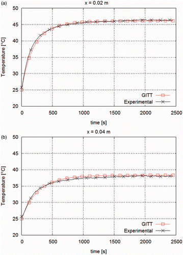
Figure 17. (a) Vertical spatial distribution of temperatures at t = 400 s and (b) vertical spatial distribution of temperatures at t = 2210 s.

6. Conclusions

In this work, we have used a combination of integral transforms for the direct problem solution and compression of the experimental data, together with Bayesian inference for the inverse problem analysis, and infrared thermography as the temperature measurement technique, for the estimation of spatially variable thermophysical properties in nanocomposites. We demonstrated the proposed methodology in experiments involving a nanocomposite plate made of polyester resin and alumina nanoparticles, with an abrupt variation in the thermophysical properties due to the abrupt variation of the filler concentration. We highlight two innovative aspects of the proposed inverse analysis, which are the representation of the unknown properties as eigenfunction expansions, with the subsequent estimation of the expansions coefficients instead of a swarm of local values, and the integral transformation along the space variable of the temperature measurements, thus compressing the experimental data into a few modes of the transformed temperatures. Furthermore, two novel aspects have been investigated here that complement the understanding of the combined inverse analysis approach. First, the use of non-informative filtering functions in the properties eigenfunction expansions allowed for the proper identification of the expected behaviour of an abrupt spatial variation, while the subsequent use of a filter with some information on this observed variability pattern provided further refinement on the predicted thermophysical properties profiles. Second, two different experimental setups were analysed, by varying the heater positioning. It has then been concluded that significant improvement can be achieved by properly choosing the heater spatial location across the region of marked spatial variation on the properties to be estimated, and thus of increased sensitivity, either based on prior information on this spatial pattern, or again in subsequent experiments aimed at refining the estimated space-variable properties.

Acknowledgements

The authors acknowledge the financial support provided by the Brazilian agencies CNPq, CAPES and FAPERJ.

References

- Lin, SH, 1992. Transient conduction in heterogeneous media, Int. Commun. Heat Mass Transfer 10 (1992), pp. 165–174.
- Qiulin, F, Xingcheng, X, Xingfang, H, and Jingkun, G, 1999. Calculating method of the equivalent thermal conductivity of functionally gradient materials, Mater. Sci. Eng. A 261 (1999), pp. 84–88.
- Fudym, O, Ladevie, B, and Batsale, JC, 2002. A seminumerical approach for heat diffusion in heterogeneous media: One extension of the analytical quadrupole method, Num. Heat Transfer, Part B: Fundamentals 42 (2002), pp. 325–348.
- Danes, F, Garnier, B, and Dupuis, T, 2003. Predicting, measuring and tailoring the transverse thermal conductivity of composites from polymer matrix and metal filler, Int. J. Thermophys. 24 (2003), pp. 771–784.
- Kumlutas, D, and Tavman, IH, 2006. A numerical and experimental study on thermal conductivity of particle filled polymer composites, J. Thermoplastic Compos. Mater. 19 (2006), pp. 441–455.
- Fudym, O, Batsale, JC, and Battaglia, JL, 2007. Thermophysical properties mapping in semi-infinite longitudinally cracked plates by temperature image processing, Inverse Probl. Sci. Eng. 15 (2) (2007), pp. 163–176.
- Fudym, O, Orlande, HRB, Bamford, M, and Batsale, JC, , Bayesian approach for thermal diffusivity mapping from infrared images processing with spatially random heat pulse heating, J. Phys. Conf. Ser. (Online), v. 135, pp. 12–42, 2008.
- Rainieri, S, Bozzoli, F, and Pagliarini, G, 2009. Effect of a hydrophobic coating on the local heat transfer coefficient in forced convection under wet conditions, Exp. Heat Transfer, 22 (3) (2009), pp. 163–177.
- Bozzoli, F, and Rainieri, S, 2011. Comparative application of CGM and Wiener filtering techniques for the estimation of heat flux distribution, Inverse Probl. Sci. Eng. 19 (4) (2011), pp. 551–573.
- Naveira-Cotta, CP, Cotta, RM, and Orlande, HRB, 2011. Inverse analysis with integral transformed temperature fields for identification of thermophysical properties functions in heterogeneous media, Int. J. Heat Mass Transfer 54 (7–8) (2011), pp. 1506–1519.
- Naveira-Cotta, CP, Orlande, HRB, and Cotta, RM, 2011. Combining integral transforms and Bayesian inference in the simultaneous identification of variable thermal conductivity and thermal capacity in heterogeneous media, ASME J. Heat Transfer 133 (11) (2011), pp. 1301–1311.
- Naveira-Cotta, CP, Orlande, HRB, and Cotta, RM, 2010. Integral transforms and Bayesian inference in the identification of variable thermal conductivity in two-phase dispersed systems, Numer. Heat Transfer, Part B: Fundamentals 57 (3) (2010), pp. 1–30.
- Kaipio, J, and Somersalo, E, 2004. Statistical and Computational Inverse Problems. Berlin: Springer-Verlag; 2004.
- Zabaras, N, 2006. "Inverse problems in heat transfer". In: Minkowycz, WJ, Sparrow, EM, and Murthy, JY, eds. Handbook of Numerical Heat Transfer. New York, NY: Wiley; 2006. pp. 525–557.
- Gamerman, D, and Lopes, HF, 2006. Markov Chain Monte Carlo: Stochastic Simulation for Bayesian Inference. Boca Raton, FL: Chapman & Hall/CRC; 2006.
- Orlande, HRB, Colaço, MJ, and Dulikravich, GS, 2008. Approximation of the likelihood function in the Bayesian technique for the solution of inverse problems, Inverse Probl. Sci. En. 16 (2008), pp. 677–692.
- Cotta, RM, 1990. Hybrid numerical-analytical approach to nonlinear diffusion problems, Num. Heat Transfer, Part B 127 (1990), pp. 217–226.
- Cotta, RM, 1993. Integral Transforms in Computational Heat and Fluid Flow. Boca Raton, FL: CRC Press; 1993.
- Cotta, RM, and Mikhailov, MD, 1997. Heat Conduction: Lumped Analysis, Integral Transforms, Symbolic Computation. New York: Wiley-Interscience; 1997.
- Cotta, RM, 1998. The Integral Transform Method in Thermal and Fluids Sciences and Engineering. New York: Begell House; 1998.
- Cotta, RM, and Mikhailov, MD, 2006. "Hybrid methods and symbolic computations". In: Minkowycz, WJ, Sparrow, EM, and Murthy, JY, eds. Handbook of Numerical Heat Transfer. New York: Wiley; 2006. pp. 493–522.
- Naveira-Cotta, CP, Cotta, RM, Orlande, HRB, and Fudym, O, 2009. Eigenfunction expansions for transient diffusion in heterogeneous media, Int. J. Heat Mass Transfer 52 (2009), pp. 5029–5039.
- Cotta, CPNaveira, Orlande, HRB, Cotta, RM, and Nunes, JS, , Integral transforms, Bayesian inference, and infrared thermography in the simultaneous identification of variable thermal conductivity and diffusivity in heterogeneous media, 14th International Heat Transfer Conference, Washington, DC, USA, August 2010.
- Knupp, DC, Naveira Cotta, CP, Ayres, JVC, Orlande, HRB, and Cotta, RM, 2010. Experimental-theoretical analysis of a transient heat conduction setup via infrared thermography and unified integral transforms, Int. Rev. Chem. Eng. 2 (2010), pp. 736–747.
- Knupp, DC, Cotta, CPNaveira, Orlande, HRB, and Cotta, RM, , Experimental identification of thermophysical properties in heterogeneous materials with integral transformation of temperature measurements from infrared thermography, Exp. Heat Transfer (in press).
- Wolfram, S, , The Mathematica Book, Version 5.2, Wolfram Media, Cambridge, 2005.
- Rainieri, S, Bozzoli, F, and Pagliarini, G, 2008. Characterization of an uncooled infrared thermographic system suitable for the solution of the 2-D inverse heat conduction problem, Exp. Thermal Fluid Sci. 32 (2008), pp. 1492–1498.
- Mark, JE, 2007. Physical Properties of Polymers Handbook. New York: Springer; 2007.
- Lewis, T, and Nielsen, L, 1970. Dynamic mechanical properties of particulate-filled polymers, J. Appl. Polymer Sci. 14 (6) (1970), pp. 1449–1471.
- Evans, W, Prasher, R, Fish, J, Meakin, P, Phelan, P, and Keblinski, P, 2008. Effect of aggregation and interfacial thermal resistance on thermal conductivity of nanocomposites and colloidal nanofluids, Int. J. Heat Mass Transfer 51 (2008), pp. 1431–1438.
- Sphaier, LA, Cotta, RM, Naveira-Cotta, CP, and Quaresma, JNN, 2011. The UNIT algorithm for solving one-dimensional convection-diffusion problems via integral transforms, Int. Commun Heat Mass Transfer 38 (5) (2011), pp. 565–571.