An inverse problem approach to stiffness mapping for early detection of breast cancer

Abstract

Early detection of breast cancer will continue to be crucial in improving patient survival rates. Our ultimate goal is to develop a system that automates, quantifies and enhances the resolution of the manual breast exam. In this study, we examine computational techniques which use breast surface force and deflection measurements to create detailed maps of the elastic modulus of the interior of the breast tissue. This approach is a reformulation of our earlier two-dimensional technique to make it more practical and we extend the approach to three dimensions. Finite element methods were used to model the tissue response (reaction force and surface displacements) to applied surface indentations. A variety of test cases with assumed tumour locations were defined, and ‘measured results’ were created. Numerical noise was added to these simulated measurements at two noise levels. A genetic algorithm was developed to identify the distribution of tissue material properties within the breast given the ‘measured’ reaction forces and surface displacements. For our two- and three-dimensional model problems, tumours as small as 1 cm could be detected reliably at a signal-to-noise ratio of 23 dB.

Keywords:

• breast cancer
• genetic algorithm
• finite elements
• inverse problem
• elastography

1. Introduction

Early detection of breast cancer will continue to be crucial in improving patient survival rates. Manual breast exams (breast palpation) and mammograms are currently the most effective and widely used early detection techniques. Unfortunately, manual breast exams are limited in their ability to detect tumours since they only produce local information about the site where the force is applied and do not provide quantitative measurements. Mammograms, while effective, expose the patient to radiation and hence routine mammograms are limited to those in specific age or risk groups. In addition, mammograms do not quantify tissue stiffness, an identifying characteristic of breast tumours. Our goal is to develop a new method for the routine early detection of tumours which exploits this stiffness difference.

It is widely agreed that cancerous tissue has an elastic modulus (stiffness) as much as 10 times that of the surrounding breast tissue 1,2. Not only this is the basis of manual breast exams, but it is also the reason many researchers have studied approaches that use MRI, CT or ultrasound measurements to create elastic modulus maps of the breast tissue. (Greenleaf et al. 1 provide a detailed review). However, because they are expensive and stressful to the patient (particularly CT/MRI), these techniques primarily address the classification of cancerous sites in patients where suspected tumours have already been identified by other early detection methods.

Our ultimate goal is to develop a system that automates, quantifies and enhances the resolution of the manual breast exam. An electro-mechanical device will gently indent the tissue surface in various locations, recording the applied force and tissue surface deflections. (Note that we record only the final applied force and deflection at each location, not their time histories.) This force/deflection data will be used with inverse techniques involving finite element methods and genetic algorithms (GAs) to provide detailed 3D maps of the elastic modulus of the interior of the breast tissue. These 3D maps could then be used to identify any suspicious sites. These maps could also provide quantitative values for comparing baseline data (which could be taken at an early age since there is no radiation or other risk to the patient) with data taken on subsequent visits, providing yet another mechanism for early identification of cancerous sites.

In practice, we anticipate that the procedure would occur as follows:

1.	The patient would lie supine on the examining table, and an electromechanical device will gently indent the breast surface in various locations.
2.	For each indentation site, the reaction forces at the indenter and the displacements over the breast tissue surface would be recorded as the ‘measured result’.
3.	A GA would be used to infer the tissue stiffness distribution in a finite element model (FEM) of the breast. Within each generation of the GA, we would a. Create ‘individuals’ each of which is a FEM of the breast, with an assumed material property distribution. b. For each of the individuals, the indentation patterns would be applied to the model and the resulting reaction forces and surface displacements would be recorded. c. Each individual would be assigned a ‘fitness’ value which indicates how closely the response of the FEM matched the ‘measured result’. d. The best individuals would be retained and allowed to mate and produce children, while the other individuals would be discarded. e. This process would be repeated for each generation of the GA.
4.	When the GA converges, the top-ranked individual's material property distribution would be reported as the stiffness distribution in the breast.

This computational study reformulates an earlier two-dimensional technique to make it more practical and extends the methods to three dimensions. In a previous work 3, we developed a set of computational algorithms and examined their performance extensively on two-dimensional model problems. However, the optimizations used to obtain convergence in this early formulation required that we impose complicated normal and tangential force patterns over the entire tissue surface – which could be difficult to implement in practice. In this study, we revise the formulation to use indentation test patterns that only require the imposition of normal displacements over small patches of the tissue surface. We have re-examined the performance of the method on the two-dimensional problems and have extended the method to three-dimensional simulations. Section 2 discusses related work in this field, Section 3 details our reformulated technique, Section 4 describes our tests and the results and Section 5 summarizes our work and suggests avenues for further development.

2. Background literature

Many authors have looked at identifying flaws (or holes) in solid materials from a non-destructive testing point of view. Because it is so closely related to our applications, the work of Schnur and Zabaras 4 is of particular interest. They demonstrated that finite element techniques, combined with a modified Levenberg-Marquardt optimization method, could be used to simultaneously identify the material properties and boundary of a circular inclusion within an otherwise homogeneous domain. They used only surface measurements, and as such their goals and approach were closely related to ours. The Levenberg–Marquardt method requires both a first and second derivative of the objective function, and so is unsuitable for our purposes, but their success suggests that our attempts may be productive.

Existing studies on identifying stiffer cancerous tissues in healthy breast tissue fall into three basic categories – methods that require the displacement field (or strain field) within the breast tissue itself, methods that measure static reaction pressures/forces on the breast surface and methods that use a sinusoidal excitation with breast surface displacement measurements.

Methods that require the displacement field within the breast tissue: Greenleaf et al. 1 provide a review of the first class of techniques, which have been explored by many researchers. These techniques are referred to by a variety of names, including ‘elastography’, ‘elasticity imaging’, ‘elastic modulus imaging’, ‘ultrafast imaging’ and ‘vibroacoustography’. The common thread in each of these methods is the use of formal inverse techniques to infer the shear modulus or Young's modulus distribution in the breast tissue from measurements of the displacement (or, alternatively, strain) throughout the interior of the breast. The methods differ in the loading used to cause the displacements (external static loads, external time-dependent loads or internal time-dependent loads), and the methods used to measure the displacements (typically ultrasound-based or magnetic resonance-based techniques).

Recent work on this approach includes studies by Barbone, Oberai, and their colleagues 5–13. They have extended their methods, which employ quasi-static displacement measurements, to nonlinear material models and have tested these techniques on tissue phantoms and in preliminary in vivo studies. Park and Maniatty 14,15 use finite elements to solve for the interpolated shear modulus field with time-dependent displacement data in the interior of the domain and the dynamic equilibrium equations. McLaughlin and her colleagues 16–20 also study solutions to the dynamic elastography problem and have progressed to preliminary in vivo testing in the liver and the spleen. Greenleaf, Fatemi, and their co-workers 21–24 employ vibro-acoustography (a dynamic response excited by ultrasound radiation forces). They have reported promising results in ex vivo studies of prostate tissue. Perrinez et al. 25 examine the ability of time-harmonic magnetic resonance elastography to reconstruct material properties for poroelastic (tofu) phantoms and find that linear elastic models are insufficient. Continuing this work, Perreard et al. 26 examine the effects of mismatches between the assumed material model and the actual material response of their phantoms. They found that treating poroelastic or anisotropic materials as linear isotropic elastic materials caused substantial errors. Eskandari et al. 27 and Guo et al. 28 have each investigated direct finite element solution techniques for elastography which promise to improve the speed of reconstructions. This first category of techniques has a rich history of contributions by many researchers 29–45.

The methods in this first group, all employ ultrasound, magnetic resonance or computed tomography techniques to measure the displacements within the breast tissue, and they require relatively sophisticated equipment (and in some cases exposure to radiation). While they show promise for characterizing and localizing already identified tumours more accurately, they are unlikely to be used for routine screening of all patients in the near future.

Methods that measure static reaction pressures/forces on the breast surface: Studies related to ‘tactile imaging’, ‘mechanical imaging’ or ‘palpation imaging’ take a fundamentally different approach. Here, a wand (similar to an ultrasound wand) is manually scanned over the breast surface. A grid of reaction pressures is measured by the wand, and the patterns overlap to form a full map of the surface reaction pressures. In her thesis, Wellman 46 gave some preliminary results on matching the surface pressure distributions to typical tumour locations, and also reported on clinical use of the scanning device. Wellman et al. 47 report on clinical scans of women preparing to undergo surgery, and hence with known breast lumps. In this case, their goal was to estimate the lump size. The estimates compared well with post-surgical lump size measurements and were more accurate than values from manual palpation or ultrasound. However, these size estimates were based on heuristics rather than a formal inverse procedure. Kaufman et al. 48 explore the use of palpation imaging as a method for documenting the breast examination. Weiss et al. 49 and Niemczyk et al. 50 report on pilot studies of a mechanical imaging device for use in detecting prostate cancer, which, like breast cancer, is often identified through manual palpation. Sarvazyan, Egorov, and their colleagues 51–56 have continued to develop this type of approach. Most recently, they reported on a clinical trial of their imager, using it to empirically classify breast cancer lumps which have already been identified by other methods. Yen et al. 57 attach both force and displacement sensors to an existing ultrasound wand and also attempt to characterize lumps which have previously been identified through ultrasound techniques.

Shih, Shih, and their co-workers 58–61 have developed a device they term a ‘piezo-electric finger’ or PEF. This is a flexible cantilever with attached force and displacement sensors which is scanned over the tissue surface. They map their results to a 1D equation to infer the tissue stiffness beneath the surface. Tissue phantom testing shows promise in characterizing lumps.

As with our proposed technique, these methods use surface measurements. However, the pressure/force measurements are only taken at the site where the forces are applied, and geometry and displacement data away from the forced locations are not recorded. Heuristic or approximate relationships is used to characterize the previously-located tumours.

Methods that use a sinusoidal excitation with breast surface displacement measurements: Haan, Chase, VanHouten, and their colleagues 62–68 have developed a third approach to the problem, which they have termed Digital Image-based Elasto-Tomography, or DIET. They use an external sinusoidal excitation of the breast surface, and use digital camera images to monitor the steady-state motion of the tissue surface. The significant computational problems associated with calculating accurate surface displacements from multiple camera images have received a substantial portion of their attention 62,63. Most recently 64,65, they present experimental and computational results from silicone phantoms: identifying stiff regions within a softer material. One of the phantoms is stacked – a soft cylinder on top of a stiff cylinder – while the other is concentric – a soft cylinder surrounding a stiff cylinder. At this stage, even for large inclusions, they are encountering difficulty in reconstructing the stiffnesses and sizes in the concentric case. Nevertheless their work is encouraging.

The DIET method involves a steady dynamic excitation in contrast to the static deformations that we envision with our technique, thus introducing tissue density as well as stiffness into the calculations. In addition, the DIET method does not make use of force information which we use in combination with the displacement information.

In summarizing this section, we would like to emphasize that our proposed approach is distinct from all three of these methods. We seek to develop inverse techniques which infer (or map) the stiffness throughout the breast tissue based only on a knowledge of quasi-static surface forces and corresponding surface displacements, systematizing the techniques used in breast palpation.

2.1. Material models and properties for breast tissues

In order to test and refine approaches to estimating the stiffness of breast tissues, we need reliable information on material models and properties of breast tissues.

Although the response of breast tissue for small strains can be modelled as incompressible linear elastic, for larger strains a nonlinear viscoelastic material model is generally considered to be more appropriate. Greenleaf et al. 1 discuss material properties for biological tissues. Krousop et al. 69 measured the moduli for breast tissue assuming a linear elastic model. They found that the modulus of some tissues varied with strain, but only for strains of the order of 20–30%. For strains up to 10% the modulus was nearly constant. Samani et al. 2,70 provide more recent extensive tissue data which included 169 tissue samples. Using a linear elastic model for the tissues, fat had a Young's modulus of 3.25 ± 0.91 kPa, which was similar to healthy fibroglandular tissue at 3.24 ± 0.61 kPa. In contrast, intermediate-grade Invasive Ductal Carcinoma (IDC) had a stiffness of 19.99 ± 4.2 kPa and high-grade IDC was 42.52 ± 12.47 kPa. They concluded that a linear elastic model was adequate for cancerous tissues. They examined this issue again 71–73, utilizing experiments to fit healthy and cancerous tissues to hyperelastic material models of various types. The nonlinear material parameters for healthy and pathological tissues showed distinct differences. In addition to their work on linear elastography methods, Barbone and Oberai and their colleagues 7,8,11, have studied nonlinear material models for elastography. They conclude that the nonlinear term in the material model is a better discriminator of tumour type (benign, cancerous). However, for our purposes it is more important that they conclude that small strain results are essentially independent of the nonlinear term and that the tumour itself rarely sees large strains, since it is embedded in substantially less stiff tissues.

Based on this work, we tested our computational methods using a linear elastic material model with a healthy tissue modulus of 3 kPa and a cancerous value of 30 kPa.

3. Numerical methods

In our new approach, we simulate the use of an indenter to impose normal displacements on patches of the tissue surface. We record the force required to impose those displacements as well as the resulting normal displacements over the remaining tissue surface. With this input data, a GA in combination with FEM is used to obtain a tissue stiffness map.

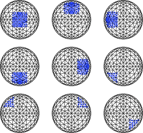
At present, we have chosen the indentation test patterns somewhat arbitrarily. Figure 1 shows the first three of the nine test patterns we used in our two-dimensional studies. The patterns involve only normal displacements and the indenter displaces a patch of the surface. (Although, we have currently chosen to indent one patch at a time, this is not a restriction on the algorithm and multiple patches could be indented simultaneously.) Similar patches are used in three-dimensions, as described in Appendix A. (In our previous work 3, we used an eigenproblem-based algorithm to optimize 2D test patterns, but that approach was not used here. In the future, we hope to extend the spirit of that optimization to these more constrained indentation test patterns.)

Figure 1. First three of the nine indentation test patterns for two-dimensional test cases.

Identifying the presence or absence of tumours within the healthy breast tissue based solely on surface measurements of force/deflection is an ‘inverse parameter estimation’ problem. Our approach to this inverse problem is to use a GA, which is basically a methodical ‘guess and check’ used to identify the tissue material property distribution that best fits our measured data:

•	Randomly create an initial population of individuals
•	For each generation • Evaluate each individual for its ‘fitness’ • Select top individuals as ‘parents’, discard others • Mate parents to create new individuals (‘children’) • Introduce mutations into some children
•	(Continue until convergence)

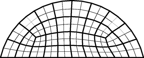
FEMs are used to evaluate individuals. Figure 2 shows 2D and 3D meshes used for individuals. Elements in the mesh are chosen to have either ‘healthy’ or ‘cancerous’ tissue, and this choice defines the individual. The finite elements themselves are nearly incompressible (ν = 0.49) displacement/pressure elements 74. (In 2D, we use the plane strain assumption.) The information about the individuals is coded into a ‘chromosome’ (Figure 3) which lists the material properties for each of the elements. Once the finite element meshes and material properties for each individual are defined, it is straightforward to apply the indentation patterns, determine the reaction forces and surface displacements for each individual, and assess their fitness.

Figure 2. Finite element meshes used to represent individuals (a) Two-dimensional mesh and (b) Three-dimensional mesh.

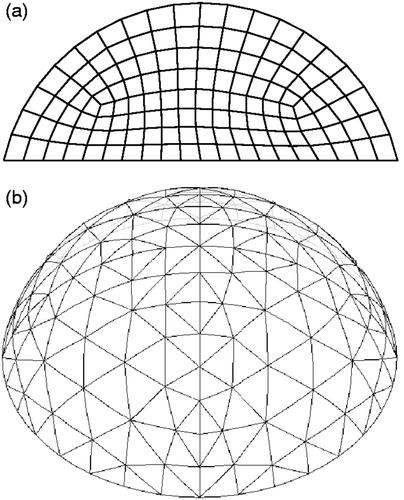
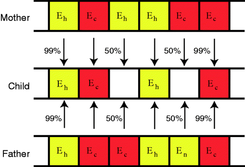
Figure 3. Chromosome used to encode material property information for each individual. (E_h is healthy modulus, E_c is cancerous modulus.)

Additional details on our methodology are given in the appendices: Appendix B discusses the GA parameters and Appendix C describes the numerical algorithms for the forward finite element problems (including the calculation of indentation forces and surface normal displacements).

4. Testing and results

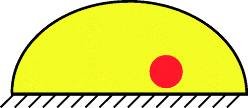
We have used simplified model problems for our testing in two and three dimensions. As indicated schematically in Figure 4, in our two-dimensional trials, we use a domain which is a circular arc with a width of 10 cm and a height of 4 cm. At the base of the domain (the breast/chest boundary), we completely restrain the tissue. In two dimensions, we assume plane strain. In three dimensions, we revolve this planar model about it's central axis.

Figure 4. Model problem geometry for two-dimensional test cases.

In order to test our algorithms, we create simulated ‘measured data’ from a more refined finite element mesh. A tumour location is assumed in this finer mesh and the indentation test patterns are applied. The reaction forces and normal displacements are recorded and white Gaussian noise is added to simulate measurement errors. Then the noisy data is downsampled to the original mesh to create the ‘measured data’. Appendix D gives details on the specific refined meshes and procedures used to create the ‘measured data’.

For these tests we allowed the GA to run for 50 generations. In preliminary testing, the algorithm had generally converged to its final solution within 10 generations, so 50 generations was considered adequate for these model studies.

The elements within the meshes are assigned to ‘clumps’ of elements and all elements within a clump are constrained to have the same material property. Figure 5 shows the 32 clumps for the two-dimensional case. This has two beneficial effects: it reduces the search space without coarsening the finite element mesh and it allows us to test our algorithms with tumours that cross clump boundaries, i.e. tumours that cannot be exactly represented in our search space. Each of the test cases presented in Sections 4.1 and 4.2 contain test tumours that cross clumps. This gives an indication of whether the algorithm can identify tumours in roughly the correct location, even when those locations do not correspond to our assumed clumps.

Figure 5. Finite element mesh showing ‘clumps’ of potential tumour elements.

In two dimensions, it is simple to create element clumps, but in three dimensions it is more challenging. We broke the three-dimensional domain into clumps by slicing the domain radially, circumferentially, and vertically so that each of the 176 clumps had approximately a 1 cm³ volume. (Appendix E describes this in more detail.)

Note that our current two-dimensional model involves 32 clumps of elements with two possible stiffnesses per element. If we were to use an exhaustive search, we would need to examine 2³² ≈ 4.3 × 10⁹ cases. Our GA uses 50 generations and 1024 individuals per generation so that we check approximately 5 × 10⁴ cases. Thus, an exhaustive search is unlikely to yield results while the GA provides an effective method for identifying the solution.

4.1. Two-dimensional results

We ran eight test cases for this two-dimensional problem, with 20 trials (implementations of noise) for each. Figure 6 shows one of the more challenging cases for a signal-to-noise ratio (SNR) of 23 dB. The actual location of the tumour is shown as a bold/green/grey outline. For this test case, we chose two sets of four elements that are diagonally adjacent to each other in the mesh. Each set of four elements is roughly 1 cm on a side. The numbers inside each shaded clump of elements indicates the number of times that clump of elements was identified as cancerous (out of the 20 trials). Since the tumours were deliberately chosen to cross the predefined element clumps, we are interested in whether the algorithm predicts cancerous elements in the vicinity of the tumour. For this case, we see some scatter in the predicted location of the tumour. However, the algorithm always chose at least two clumps of four elements as cancerous, and 12/20 times the algorithm identified three clumps of four elements as cancerous. Figure 7 displays the results for a variety of tumour locations including the result from Figure 6. The majority of the test cases show very little scatter.

Figure 6. Challenging test case for 20 trials with SNR = 23 dB. Bold/green/grey lines show the location of the test tumours, and the numbers in the elements indicate how many times the algorithm identified that clump of elements as a tumour. For every trial at least eight elements were identified as cancerous.

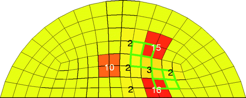
Figure 7. Results for eight different test cases with SNR = 23 dB and 20 trials. Bold/green/grey lines show the location of the test tumours, and the numbers in the elements indicate how many times the algorithm identified that clump of elements as a tumour. For every trial containing a test tumour at least four elements were identified as cancerous.

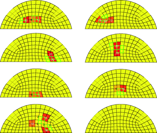
If we decrease the SNR to 20 dB the scatter in the results becomes more pronounced. However, in all cases considered at both SNRs, if there was a tumour present a tumour was always indicated, and if there was no tumour present, no tumour was indicated.

4.2. Three-dimensional results

We tested seven cases with tumours and one tumour-free case in three dimensions. Figure 8 shows a typical prediction (red/black) and the true tumour location (bold/green/grey) for a single 23 dB noise trial. In this case, the tumour was roughly a centimeter in each dimension and it crossed two clumps in the finite element mesh. The predicted location is quite a reasonable approximation to the true location. We also ran 19 other noise implementations for this example, and in all cases there was a tumour predicted that was in a clump that overlapped the true location. (The solution shown in Figure 8 is the most common solution, occurring in 11 out of 20 trials.)

Figure 8. Typical result (Test A) at SNR = 23 dB. The true tumour crosses two clumps, adjacent to the chest wall and tissue centerline. True tumour is shown in bold/green/grey and prediction is red/black. True tumour volume is 0.96 cm³. (a) Bottom view and (b) Side view.

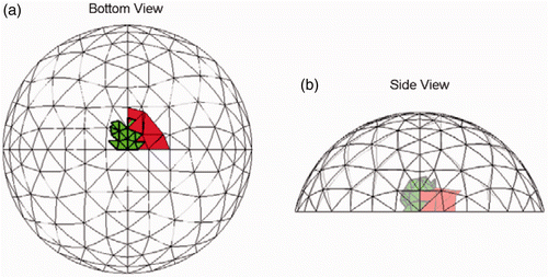
Figures 9–14 show similar results for the other six test cases with tumours. Each of these test cases has tumours that have a volume of approximately 1 cm³ and the figures show the most common result. We ran a total of 20 noise implementations at SNR = 23 dB for each of these examples and in all cases there was a tumour predicted that was in a clump that overlapped the true location. We also ran a tumour-free case which correctly reported no cancer in all 20 trials.

Figure 9. Result for Test B (20/20 trials) at SNR = 23 dB. The true tumour crosses eight clumps. True tumour is shown in bold/green/grey and prediction is red/black. True tumour volume is 1.02 cm³. (a) Bottom view and (b) Side view.

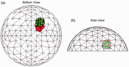
Figure 10. Result for Test C (20/20trials) at SNR = 23 dB. The true tumour crosses eight clumps. True tumour is shown in bold/green/grey and prediction is red/black. True tumour volume is 1.13 cm³. (a) Bottom view and (b) Side view.

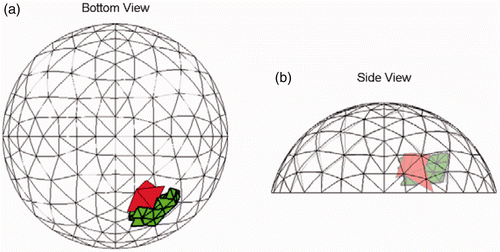
Figure 11. Most common (9/20 trials) result for Test D at SNR = 23 dB. The true tumour crosses four clumps. True tumour is shown in bold/green/grey and prediction is red/black. True tumour volume is 0.99 cm³. (a) Bottom view and (b) Side view.

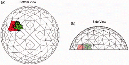
Figure 12. Most common (16/20 trials) result for Test E at SNR = 23 dB. Each of the sites in the true tumour crosses eight clumps. True tumour is shown in bold/green/grey and prediction is red/black. True tumour volume is 1.92 cm³, divided roughly equally between the two sites. (a) Bottom view and (b) Side view.

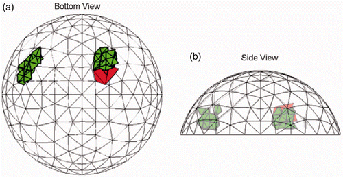
Figure 13. Result for Test F (20/20 trials) at SNR = 23 dB. The true tumour crosses eight clumps. True tumour is shown in bold/green/grey and prediction is red/black. True tumour volume is 2.07 cm³. (a) Bottom view and (b) Side view.

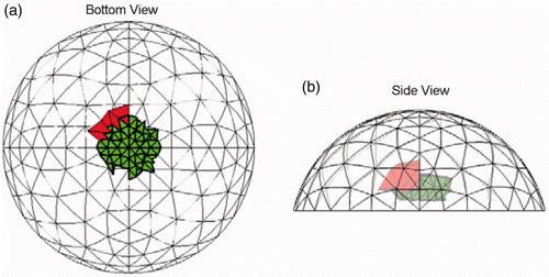
Figure 14. Result for Test G (20/20 trials) at SNR = 23 dB. The true tumour crosses twenty-two clumps. True tumour is shown in bold/green/grey and prediction is red/black. True tumour volume is 2.10 cm³. (a) Bottom view and (b) Side view.

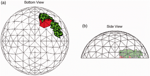
If we repeat these tests at a SNR of 20 dB, we find that the algorithm fails to identify a tumour in one of 20 trials on Test A. Tests B–F still identify tumours in all 20 trials, and the tumour-free test still correctly reports no cancer in all 20 trials. Hence, the algorithm is no longer reliable when the SNR drops to 20 dB.

Based on these results, even deep tumours as small as 1 cm can be detected reliably for these model problems at a SNR of 23 dB. To put this in context, The American Joint Committee on Cancer 75 grades cancers in part by their tumour size. Breast cancer tumours less than 2 cm where the cancer has not spread to other sites are collected into the lowest risk group for invasive cancers with a relative 5 year survival rate of 100% 76.

5. Summary and future work

We have developed new computational techniques which use breast surface force and deflection measurements to create maps of the elastic modulus of the interior of the breast tissue. A GA in combination with finite element methods was used to solve this inverse problem. A variety of tumour locations were assumed for two- and three-dimensional model problems, and ‘measured results’ were created with numerical noise added to simulate measurement errors. For these simplified test cases, tumours as small as 1 cm could be detected reliably when the SNR was 23 dB. When a tumour was present, a tumour was always detected. When a tumour was absent, the algorithm always correctly reported no cancer.

While these results are promising, there are a number of limitations in the current computational algorithm that will need to be explored in future work. In two dimensions, the geometry we chose can scale to other domain sizes – the stiffness matrix for a 10 cm by 4 cm domain is the same as that for a 15 cm by 6 cm domain. In three dimensions, this is no longer true and a variety of breast sizes will need to be tested. We will also need to explore the influence of how we model the boundary condition at the breast-chest interface on our ability to resolve the tumours. Most importantly, we have assumed that the tissues are either healthy or cancerous and have assumed that we know the values of those tissue stiffnesses. We will need to introduce ranges of tissue properties.

There are a number of factors affecting computational efficiency that will also need to be addressed. Although our results are promising we have not made any attempt to optimize either the indentation patterns or the fitness function. In addition, we have not studied termination criteria for the GA.

Our ultimate goal is to develop a system that automates, quantifies and enhances the resolution of the manual breast exam. In addition to improvements in the computational studies, we are working towards validation of our computational approaches through tissue phantom experiments. These experiments will help to define what measurement errors (magnitudes and types) can reasonably be expected for such a system.

Acknowledgements

This work used the Extreme Science and Engineering Discovery Environment (XSEDE), which is supported by National Science Foundation grant number OCI-1053575. Resources were obtained through the Texas Advanced Computing Center at The University of Texas at Austin.

Notes

1. Element centers were calculated using the MATLAB^TM ‘incenters’ function from the first four nodes of each element.

Appendix

Figure A1 shows the nine indentation test patterns for the three-dimensional meshes. In each indentation test pattern all of the nodes (marked with a ‘*’) within the patch are displaced a normal distance of 0.5 cm into the surface. For each node the normal is computed as described in Appendix C.

Figure A1. Nine indentation test patterns for three-dimensional test cases.

Appendix

Our goal in the GA is to determine how to assign material properties (E_h and E_c) to elements in the finite element mesh in order to ‘best’ match the ‘measured data’ under the same surface loadings. Section 3 described the general process and in this appendix we give details on the definition of the individuals/population, fitness function and parent selection, mating and mutation.

B.1. Individuals/population

Each individual is defined by a chromosome consisting of one gene for the stiffness (E_h and E_c) of each element in the finite element mesh. In our 2D simulations, we used 1024 individuals of which 32 were selected as parents. Each pair of parents was used to create 62 children. Table B1 lists these values as well as those for the 3D analyses. Our numerical experiments indicated that our application converged more quickly with few parents and many children per parent. In the first generation the population was initialized with one tumour-free individual and the remainder of the population was generated randomly.

Table 1. Parameter settings for 2D and 3D GA.

Parameter	Value for 2D simulations	Value for 3D simulations
Total individuals	1024	2560
Parents	32	16
Children/parent pair	62	318

B.2. Fitness function and parent selection

‘Fitness’ is a measure of how well the individual's force and displacement responses match the measured (true) force and displacement responses for the same imposed surface displacements, and only individuals with the best fit (small numbers) are are allowed to reproduce. The fitness function we chose for both 2D and 3D analyses was (1) where

CCave =	=	correlation coefficient between measured normal displacement and individual normal displacement, averaged over all load cases
δnorm =	=
δ =	=	sum of absolute error between measured normal displacement and individual normal displacement (summed over all load cases)
δ1 =	=	largest value of δ encountered in first generation
fnorm =	=
f =	=	sum of absolute error between measured normal force and individual normal force (summed over all load cases)
f1 =	=	largest value of f encountered in first generation
Rnorm =	=
Rave =	=	average radius of tumour
R1 =	=	largest value of Rave encountered in first generation

The first term in Equation (B1) is intended to account for the shape of the displacement profile since the correlation coefficient is independent of amplitude. The second and third terms account for the amplitudes of the displacements and the reaction forces, respectively. The last term is included to create a small bias towards compact tumours. We did not attempt to optimize this fitness function at this stage, although we anticipate that we will be able to improve our ability to resolve the stiffness map in the future by studying alternative fitness functions.

In each generation, unique individuals with the smallest fitness function are chosen as parents and the rest of the population is discarded. Two individuals are identified as non-unique if their fitness functions are within a tolerance of 10⁻⁵ and they have equal numbers of cancerous genes.

B.3. Mating

Once the parents have been identified, they are mated in pairs to produce children. We use the cost weighting method described in Haupt and Haupt 77 to assign parent pairs.

Figure B1 indicates the mating process. If both parents have the same gene the child has a 99% chance of having that gene. If the parents have different genes then the child has an equal chance to get the mother's gene or the father's gene.

Figure B1. Mating parents to create children.

Both the parents and the children are retained for the next generation.

B.4. Mutation

Once the children are created, mutations are introduced. (Only the children, not the parents, receive mutations.) A random number of children, up to 50%, are selected for mutation. On those selected a random number of genes, up to 50%, are mutated. A mutation consists of changing the gene from healthy to cancerous or cancerous to healthy.

Appendix

We wish to impose only normal surface displacements as test patterns and then ‘measure’ the normal surface displacements over the entire surface as well as the force required to create the imposed surface displacements. We have used Lagrange multipliers to impose the normal surface displacements in a pointwise fashion on the tissue surface.

Consider an ordinary finite element stiffness matrix with normal surface displacements imposed by Lagrange multipliers: (2) where

KUU =	=	Stiffness matrix for tissue before any normal surface displacements are applied
BUf =	=	Matrix of tissue surface normals
U =	=	Vector of tissue nodal displacements (global Cartesian coordinate system)
f =	=	Vector of Lagrange multipliers (normal forces) required to impose normal displacements
δ =	=	Vector of imposed normal surface displacements

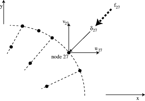
B_Uf is probably the most confusing entry in this matrix equation. It contains the surface normals used to enforce pointwise constraints on the Cartesian nodal displacements. Consider node 27 (an arbitrary node) on the two-dimensional tissue surface shown schematically in Figure C1. It has x–y Cartesian nodal displacements u₂₇ and v₂₇ which are entries in the vector U. We wish to require that it have a normal displacement δ₂₇ which will be imposed by a Lagrange multiplier f₂₇. The relationship between these variables is given by (3) where n_x and n_y are the unit inward normals at this surface node and f_x and f_y are the components of the force required to impose the normal displacement. The f_x and f_y are automatically balanced by the internal forces generated by the elements used to assemble K_UU and are never calculated. B_Uf consists of the matrix assembly of all of the contributions (4) from each of the surface nodes.

Figure C1. Applying the nodal surface constraints.

Next, we must define how we will compute the surface normal for the nodes. For mid-side nodes in two-dimensional analyses, there is not too much ambiguity – we simply use the normal to the line element evaluated at that node. For nodes connected to two elements in 2D, we use the average of the normals calculated in each element. In three dimensions, all six of the nodes on our surface elements are attached to additional elements. We use the average of the normals calculated over all of the elements to which the node is attached. The normal within an element is calculated as the cross product of two vectors evaluated at the node: one tangent to the surface and parallel to the element side and one tangent to the surface and perpendicular to the element side.

The term K_UU in Equation C1 depends only on the material properties in the tissue and not on the particular displacement test pattern. Hence, we solve for U and f in two stages:

1.	Calculate by doing a partial forward reduction of the full matrix.
2.	For each displacement test pattern, a. eliminate the f degrees of freedom which are not active for this displacement test pattern, b. for the remaining dofs, complete the forward reduction of the matrix and the load vector, and c. backsubstitute to solve for U and f for this displacement test pattern.

C.1. Calculating normal displacements over the entire tissue surface

For each U and f solution, we must find the normal displacements everywhere on the tissue surface. This is simply done by multiplying the previously calculated matrix of surface normals by the displacements U: (5)

C.2. Calculating normal reaction forces due to applied displacements

The reaction forces at the surface where the displacements are prescribed are also calculated after the displacements everywhere in the tissue domain have been calculated. We make the calculation for each domain element that is in contact with the prescribed surface. In what follows we describe the methods we applied for the two-dimensional models in detail.

As originally formulated, our two-dimensional element 74 was a nine-node element with a linear discontinuous pressure field. We have implemented it as an eight-node element with the ninth node and the pressure degrees of freedom condensed out at the element level, before the global matrix is assembled.

For each of these domain elements, we first create the displacement portion of the stress-strain constitutive matrix, C_uu (6) where , E = Young's Modulus, and ν = Poisson's ratio.

Next, a ninth node is created at the center of the element. Since the ninth node should lie at r = 0, s = 0, we use the eight-node isoparametric shape functions evaluated there to write (7) and (8) with x_i and y_i the local nodal coordinates.

Now, using nine-node isoparametric shape functions (h_i), we create the matrices that comprise the stiffness. (9) (10) (11)

The element matrix is then created from (12) where (13) (14) (15) and (16) Here the determinant of the Jacobian, |J|, of the element is computed in the usual way for isoparametric elements 78.

We seek to calculate the forces that would have been applied to the nodes to create the displacements we now know. For a single element, we could write (17) Because we condensed the ninth node and pressure degrees of freedom out of the stiffness matrix before assembling the global matrix 79, we only have the nodal displacements on the eight nodes. Hence, we again need to condense the element stiffness matrix: (18) Note that the force on the ninth node must be zero, so no information about the forces is lost in this process.

Once the nodal forces for the element have been calculated, we select the nodes at the surface of the domain where the displacements were prescribed. At each of these nodes, we identify the local normal to the element surface and use that to find the normal force at the node. The sum of the normal forces for the element is recorded as the force for that element.

This procedure is repeated for each element that had a normal displacement imposed on it. The forces are recorded for comparison with ‘measured data’ on the surface forces.

In our three-dimensional analyses, we use an analogous procedure to find the force patterns, although the elements are ten-node tetrahedrons with a single pressure degree of freedom and only the pressure degree of freedom is condensed out at the element level.

Appendix

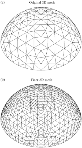
First, a finer mesh is created by refining the original mesh. Figure D1 shows the original and finer meshes for the two-dimensional case and Figure D2 shows the corresponding information for the three-dimensional case. The applied displacement test functions from the original mesh are mapped to the finer mesh and a finite element solution is computed for each of the test functions. The normal surface displacements are extracted, and the element surface force patterns required to cause each of the applied displacements are also extracted.

Figure D1. Finer mesh used to create measured data for original mesh in two dimensions. (a) Original 2D mesh and (b) Finer 2D mesh.

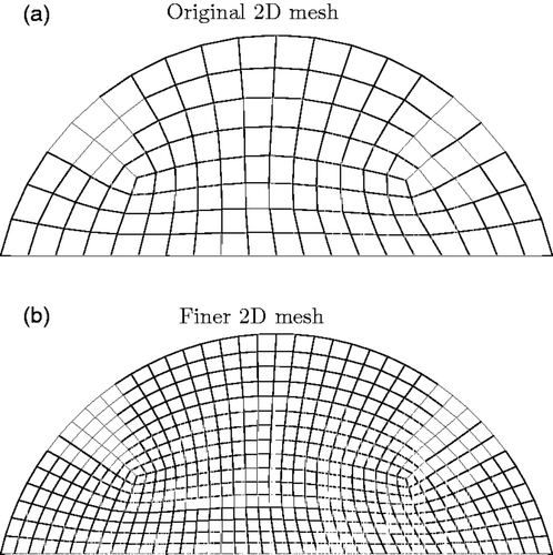
Figure D2. Finer mesh used to create measured data for original mesh in three dimensions. (a) Original 2D mesh and (b) Finer 2D mesh.

Next, random Gaussian noise with a specific SNR is added to the displacement and force patterns. The SNR is defined as (19) Here, σ_s is the standard deviation of the signal and σ_n is the standard deviation for the noise. For the displacements, the standard deviation of the signal is computed as a single value over all of the true displacement patterns, but excluding the prescribed displacement values. For the forces, the standard deviation of the signal is computed as a single value over all of the true force patterns, including only locations where displacements were prescribed. For each displacement and force pattern, 20 different data sets were created by adding noise.

To create the ‘measured data’ we downsample these noisy data sets to the original mesh. The normal surface displacement data for the original mesh is simply selected from the values for the closest surface nodes in the finer mesh. To map the noisy force values to the original mesh, we accumulate the forces in the finer mesh, i.e. in 2D we sum up the forces on the two finer surface elements to create a ‘measured’ force pattern on one surface element in the original mesh.

Appendix

As mentioned earlier, the elements within the meshes are assigned to ‘clumps’ of elements and elements within a clump are constrained to have the same material property in the GA. In our two-dimensional meshes, it is easy to create elements clumps, as shown previously in Figure 5.

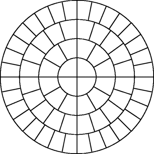
In our three dimensional meshes the clumping process is more difficult. We seek clumps of roughly 1 cm³ in order to allow us to identify tumours of this size. The mesh volume is 186.3 cm³ and so we used 176 clumps each with an average volume of 1.059 cm³. The clumps were assigned by dividing the mesh into regions radially, circumferentially, and vertically. Figure E1 shows a top view of the three-dimensional domain with the radial and circumferential region boundaries. The radial coordinates for the region boundaries were set at intervals of 1.25 cm and the circumferential boundaries were evenly spaced within each quadrant. Although the boundaries are regular, the mesh itself is unstructured. An element was assigned to a clump if its center1 fell within the region boundaries. Within each radial and circumferential region we established vertical boundaries by manually adjusting the cut-off heights so that the total volume of the elements within each clump was approximately 1 cm³. The final distribution of the element volumes was such that the smallest clump volume was 0.57 cm³, the largest was 1.70 cm³, and the standard deviation was 0.24 cm³.

Figure E1. Radial and circumferential boundaries for three-dimensional clumps.

References

- Greenleaf, JF, Fatemi, M, and Insana, M, 2003. Selected methods for imaging elastic properties of biological tissues, Annu. Rev. Biomed. Eng. 5 (2003), pp. 57–78.
- Samani, A, Zubovits, J, and Plewes, D, 2007. Elastic moduli of normal and pathological human breast tissues: An inversion-technique-based investigation of 169 samples, Phys. Med. Biol. 52 (2007), pp. 1565–1576.
- Olson, LG, and Throne, RD, 2010. Numerical simulation of an inverse method for tumour size and location estimation, Inverse Probl. Sci. Eng. 18 (2010), pp. 813–834.
- Schnur, DS, and Zabaras, N, 1992. An inverse method for determining elastic material properties and a material interface, Int. J. Numer. Methods Eng. 33 (1992), pp. 2039–2057.
- Barbone, PE, and Gokhale, NH, 2004. Elastic modulus imaging: On the uniqueness and nonuniqueness of the elastography inverse problem in two dimensions, Inverse Probl. 20 (2004), pp. 283–296.
- Barbone, PE, and Oberai, AA, 2007. Elastic modulus imaging: Some exact solutions of the compressible elastography inverse problem, Phys. Med. Biol. 52 (2007), pp. 1577–1593.
- Goenezen, S, Barbone, P, and Oberai, AA, 2011. Solution of the nonlinear elasticity imaging inverse problem: The incompressible case, Comput. Methods Appl. Mech. Eng. 200 (2011), pp. 1406–1420.
- Gokhale, NH, Barbone, PE, and Oberai, AA, 2008. Solution of the nonlinear elasticity imaging inverse problem: The compressible case, Inverse Probl. 24 (045010) (2008), pp. 1–26.
- Oberai, AA, Gokhale, NH, and Feijoo, GR, 2003. Solution of inverse problems in elasticity imaging using the adjoint method, Inverse Probl. 19 (2003), pp. 297–313.
- Oberai, AA, Gokhale, NH, Doyley, MM, and Bamber, JC, 2004. Evaluation of the adjoint equation based algorithm for elasticity imaging, Phys. Med. Biol. 49 (2004), pp. 2955–2974.
- Oberai, AA, Gokhale, NH, Goenezen, S, Barbone, PE, Hall, TJ, Sommer, AM, and Jiang, J, 2009. Linear and nonlinear elasticity imaging of soft tissue in vivo: Demonstration of feasibility, Phys. Med. Biol. 54 (2009), pp. 1191–1207.
- Richards, MS, Barbone, PE, and Oberai, AA, 2009. Quantitative three-dimensional elasticity imaging from quasi-static deformation: A phantom study, Phys. Med. Biol. 54 (2009), pp. 757–779.
- Rivas, C, Barbone, PE, and Oberai., AA, , Divergence of finite element formulations for inverse problems treated as optimization problems. J. Phys.: Conf. Ser., 135(012088) (2008), pp. 1–8.
- Park, E, and Maniatty, AM, 2006. Shear modulus reconstruction in dynamic elastography: Time harmonic case, Phys. Med. Biol. 51 (2006), pp. 3697–3721.
- Park, E, and Maniatty, AM, 2009. Finite element formulation for shear modulus reconstruction in transient elastography, Inverse Probl. Sci. Eng. 17 (5) (2009), pp. 605–626.
- Lin, K, and McLaughlin, J, 2009. An error estimate on the direct inversion model in shear stiffness imaging, Inverse Probl. 25 (075003) (2009), pp. 1–19.
- Lin, K, McLaughlin, J, and Zhang, N, 2009. Log-elastographic and non-marching full inverseion schemes for shear modulus recovery from single frequency elastographic data, Inverse Probl. 25 (075004) (2009), pp. 1–24.
- McLaughlin, J, and Renzi, D, 2006. Shear wave speed recovery in transient elastography and super- sonic imaging using propagating fronts, Inverse Probl. 22 (2006), pp. 681–706.
- McLaughlin, J, and Renzi, D, 2006. Using level set based inversion of arrival times to recover shear wave speed in transient elastography and supersonic imaging, Inverse Probl. 22 (2006), pp. 707–725.
- McLaughlin, JR, Zhang, N, and Manduca, A, 2010. Calculating tissue shear modulus and pressure by 2D log-elastographic methods, Inverse Probl. 26 (085007) (2010), pp. 1–25.
- Alizad, A, Wold, LE, Greenleaf, JF, and Fatemi, M, 2004. Imaging mass lesions by vibro-acoustography: Modeling and experiments, IEEE Trans. Med. Imaging 23 (9) (2004), pp. 1087–1093.
- Brigham, JC, Aquino, W, Mitri, FG, Greenleaf, JF, and Fatemi, M, 2007. Inverse estimation of viscoelastic material properties for solid immersed in fluids using vibroacoustic techniques, J. Appl. Phys. 101 (2007), pp. 1–14.
- Mitri, FG, Davis, BJ, Alizad, A, Greenleaf, JF, Wilson, TM, Mynderse, LA, and Fatemi, M, 2008. Prostate cryotherapy monitoring using vibroacoustography: Preliminary results of an ex-vivo study and technical feasibility, IEEE Trans. Biomed. Eng. 55 (11) (2008), pp. 2584–2592.
- Zhang, X, Zeraati, M, Kinnick, RR, Greenleaf, JF, and Fatemi, M, 2007. Vibration mode imaging, IEEE Trans. Med. Imaging 26 (6) (2007), pp. 843–852.
- Perrinez, PR, Kennedy, FE, Van Houten, EEW, and Weaver, JB, 2009. Modeling of soft poroelastic tissue in time-harmonic MR elastography, IEEE Trans. Biomed. Eng. 56 (3) (2009), pp. 598–608.
- Perreard, IM, Pattison, AJ, Doyley, M, McGarry, MJJ, Barani, Z, Van Houten, EEW, Weaver, JB, and Paulsen, KD, 2010. Effects of frequency- and direction-dependent elastic materials on linearly elastic MRE image reconstructions, Phys. Med. Biol. 55 (2010), pp. 6801–6815.
- Eskandari, H, Salcudean, SE, Rohling, R, and Bell, I, 2011. Real-time solution of the finite element inverse problem of viscoelasticity, Inverse Probl. 27 (085002) (2011), pp. 1–16.
- Guo, Z, You, S, Wan, X, and Bicanic, N, 2010. A FEM-based direct method for material reconstruction inverse problem in soft tissue elastography, Comput. Struct. 88 (2010), pp. 1459–1468.
- Doyley, MM, Srinivasan, S, Dimidenko, E, Soni, N, and Ophir, J, 2006. Enhancing the performance of model-based elastography by incorporating additional a priori information in the modulus reconstruction process, Phys. Med. Biol. 51 (2006), pp. 95–112.
- Fehrenbach, J, Masmoudi, M, Souchon, R, and Trompette, P, 2006. Detection of small inclusions by elastography, Inverse Probl. 22 (2006), pp. 1055–1069.
- Harrigan, TP, and Konofagu, EE, 2004. Estimation of material elastic moduli in elastography: A local method, and an investigation of poisson's ratio sensitivity, J. Biomech. 37 (2004), pp. 1215–1221.
- Haw, LLiew, and Pinksy, PM, 2005. Recovery of shear modulus in elastography using an adjoint method with b-spline representation, Finite Elem. Anal. Des. 41 (2005), pp. 778–799.
- Liu, HT, Sun, LZ, Wang, G, and Vannier, MW, 2003. Analytic modelling of breast elastography, Med. Phys. 30 (9) (2003), pp. 2340–2349.
- Liu, Y, Sun, LZ, and Wang, G, 2005. Tomography-based 3-D anisotropic elastography using boundary measurements, IEEE Trans. Med. Imaging 24 (10) (2005), pp. 1323–1333.
- Miga, MI, 2003. A new approach to elastography using mutual information and finite elements, Phys. Med. Biol. 48 (2003), pp. 467–480.
- Ou, JJ, Ong, RE, Yankeelov, TE, and Miga, MI, 2008. Evaluation of 3D modality-independent elastography for breast imaging: A simulation study, Phys. Med. Biol. 53 (2008), pp. 147–163.
- Plewes, DB, Bishop, J, Samani, A, and Sciarretta, J, 2000. Visualization and quantification of breast cancer biomechanical properties with magnetic resonance elastography, Phys. Med. Biol. 45 (2000), pp. 1591–1610.
- Samani, A, Bishop, J, and Plewes, DB, 2001. A constrained modulus reconstruction technique for breast cancer assessment, IEEE Trans. Med. Imaging 20 (9) (2001), pp. 877–885.
- Sarvazyan, AP, Rudenko, OV, Swanson, SD, Fowlkes, JB, and Emelianov, SY, 1998. Shear wave elasticity imaging: A new ultrasonic technology of medical diagnostics, Ultrasound Med. Biol. 24 (9) (1998), pp. 1419–1435.
- Sinkus, R, Tanter, M, Xydeas, T, Catheline, S, Bercoff, J, and Fink, M, 2005. Viscoelastic shear properties of in vivo breast lesions measured by MR elastography, Magn. Reson. Imaging 23 (2005), pp. 159–165.
- Sridhar, M, Liu, J, and Insana, MF, 2007. Viscoelasticity imaging using ultrasound: Parameters and error analysis, Phys. Med. Biol. 52 (2007), pp. 2425–2443.
- Thitaikumar, A, Mobbs, LM, Kraemer-Chant, CM, Garra, BS, and Ophir, J, 2008. Breast tumour classification using axial shear strain elastography: A feasibility study, Phys. Med. Biol. 53 (2008), pp. 4809–4823.
- Van Houten, EEW, Doyley, MM, Kennedy, FE, Weaver, JB, and Paulsen, KD, 2003. Initial in vivo experience with steady-state subzone-based MR elastography of the human breast, J. Magn. Reson. Imaging 17 (2003), pp. 72–85.
- Washington, CW, and Miga, MI, 2004. Modality independent elastography (MIE): A new approach to elasticity imaging, IEEE Trans. Med. Imaging 23 (9) (2004), pp. 1117–1128.
- Zhu, Y, Hall, TJ, and Jiang, J, 2003. A finite-element approach for Young's modulus reconstruction, IEEE Trans. Med. Imaging 22 (7) (2003), pp. 890–901.
- Wellman, PS, "Tactile imaging". In: Ph.D. thesis. Harvard University, 1999. Available at http://biorobotics.harvard.edu/publications.html.
- Wellman, PS, Dalton, EP, Krag, D, Kern, KA, and Howe, RD, 2001. Tactile imaging of breast masses, Arch. Surg. 136 (2001), pp. 204–208.
- Kaufman, CS, Jacobsen, L, Bachman, BA, and Kaufman, LB, 2006. Digital documentation of the physical examination: Moving the clinical breast exam to the electronic medical record, Am. J. Surg. 192 (4) (2006), pp. 444–449.
- Weiss, RE, Hartanto, V, Perrotti, M, Dummings, KB, Bykanov, AN, Egorov, V, and Sobolevsky, SA, 2001. In vitro trial of the pilot prototype of the prostate mechanical imaging system, Urology 58 (6) (2001), pp. 1059–1063.
- Niemczyk, P, Cummings, KB, Sarvazyan, AP, Bancila, E, Ward, WS, and Weiss, RE, 1998. Correlation of mechanical imaging and histopathology of radical prostatectomy specimens: A pilot study for detecting breast cancer, J. Urol. 160 (1998), pp. 797–801.
- Egorov, V, and Sarvazyan, AP, 2008. Mechanical imaging of the breast, IEEE Trans. Med. Imaging 27 (9) (2008), pp. 1275–1287.
- Egorov, V, van Raalte, H, and Sarvazyan, AP, 2010. Vaginal tactile imaging, IEEE Trans. Biomed. Eng. 57 (7) (2010), pp. 1736–1744.
- Egorov, V, Tsyuryupa, S, Kanilo, S, Kogit, M, and Saravazyan, A, 2008. Soft tissue elastometer, Med. Eng. Phys. 30 (2008), pp. 206–212.
- Egorov, V, Kearney, T, Pollak, SB, Rohatgi, C, Sarvazyan, N, Airapetian, S, Browning, S, and Sarvazyan, A, 2009. Differentiation of benign and malignant breast lesions by mechanical imaging, Breast Cancer Res. Treat. 118 (1) (2009), pp. 67–80.
- Helvie, MA, Carson, PL, Saravazyan, A, Thorson, N, Egorov, V, and Roubidoux, MA, 2003. Mechanical imaging of the breast: A pilot trial, Ultrasound Med. Biol. 29 (5S) (2003), p. S112.
- Kearney, TJ, Airpetian, A, and Sarvazyan, A, 2004. Tactile breast imaging to increase the sensitivity of breast examination, J. Clin. Oncol. 22 (14S) (2004), p. 1037.
- Yen, P-L, Chen, D-R, Yeh, K-T, and Chu, P-Y, 2011. Development of a stiffness measurement accessory for ultrasound in breast cancer diagnosis, Med. Eng. Phys. 33 (9) (2011), pp. 1108–1119.
- Szewczyk, ST, Shih, WY, and Shih, WH, 2006. Palpationlike soft-material elastic modulus measurement using piezoelectric cantilevers, Rev. Sci. Instrum. 77 (044302) (2006), pp. 1–8.
- Yegingil, H, Shih, WY, and Shih, WH, 2007. All-electrical indentation shear modulus and elastic modulus measurement using a piezoelectric cantilever with a tip, J. Appl. Phys. 101 (054510) (2007), pp. 1–10.
- Yegingil, H, Shih, WY, and Shih, WH, 2007. Probing elastic tissue modulus and depth of bottom-supported inclusions in model tissues using piezoelectric cantilevers, Rev. Sci. Instrum. 78 (115101) (2007), pp. 1–6.
- Yegingil, H, Shih, WY, and Shih, WH, 2010. Probing model tumour interfacial properties using piezoelectric cantilevers, Rev. Sci. Instrum. 81 (095104) (2010), pp. 1–9.
- Hann, CE, Chase, JG, Chen, X, Berg, C, Brown, RG, and Elliot, RB, 2009. Strobe imaging system for digital image-based elasto-tomography breast cancer screening, IEEE Trans. Ind. Electron. 56 (8) (2009), pp. 3195–3202.
- Hii, AJH, Hann, CE, Chase, JG, and Van Houten, E, 2006. Fast normalized cross correlation for motion tracking using basis functions, Comput. Methods Prog. Biomed. 82 (2006), pp. 144–156.
- Peters, A, Chase, JG, and Van Houten, EEW, 2008. Digital image elasto-tomography: Combinatorial and hybrid optimization algorithms for shape-based elastic property reconstruction, IEEE Trans. Biomed. Eng. 55 (11) (2008), pp. 2575–2583.
- Peters, A, Chase, JG, and Van Houten, EEW, 2009. Estimating elasticity in heterogeneous phantoms using digital image elasto-tomography, Med. Biol. Eng. Comput. 47 (2009), pp. 67–76.
- Peters, A, Milsant, A, Rouze, J, Ray, L, Chase, JG, and Van Houten, E, 2004. Digital image-based elasto-tomography: Proof of concept studies for surface based mechanical property reconstruction, JOSE Int. J. 47 (4) (2004), pp. 1117–1123.
- Peters, A, Wortmann, S, Elliott, R, Staiger, M, Chase, JG, and Van Houten, E, 2005. Digital image-based elasto-tomography: First experiments in surface based mechanical property estimation of gelatine phantoms, JOSE Int. J. 48 (4) (2005), pp. 562–569.
- Peters, A, Uwe-Berger, H, Chase, JG, and Van Houten, EEW, 2006. Digital image-based elasto- tomography: Non-linear mechanical property reconstruction of homogeneous gelatine phantoms, Int. J. Inform. Syst. Sci. 2 (4) (2006), pp. 512–521.
- Krouskop, TA, Wheeler, TM, Kallel, F, Garra, BS, and Hall, T, 1998. Elastic moduli of breast and prostate tissues under compression, Ultrason. Imaging 20 (1998), pp. 260–274.
- Samani, A, and Plewes, D, 2007. An inverse problem solution for measuring the elastic modulus of intact ex vivo breast tissue tumours, Phys. Med. Biol. 52 (2007), pp. 1247–1260.
- Mehrabian, H, Campbell, G, and Samani, A, 2010. A constrained reconstruction technique of hyperelasticity parameters for breast cancer assessment, Phys. Med. Biol. 55 (2010), pp. 7489–7508.
- O'Hagan, JJ, and Samani, A, 2008. Measurement of the hyperelastic properties of tissue slices with tumour inclusion, Phys. Med. Biol. 53 (2008), pp. 7087–7106.
- O'Hagan, JJ, and Samani, A, 2009. Measurement of the hyperelastic properties of 44 pathological ex vivo breast tissue samples, Phys. Med. Biol. 54 (2009), pp. 2257–2569.
- Sussman, TD, On the finite element analysis of incompressible solids, Ph.D. thesis, Massachusetts Institute of Technology, 1987. Available at http://hdl.handle.net/1721.1/14923.
- American Cancer Society, (2008). Available at: http://www.cancer.org/.
- Ries, LAG, Young, JL, Keel, GE, Eisner, MP, Lin, YD, and Horner, eds., M-J, 2007. SEER Survival Monograph: Cancer survival among adults: U.S. SEER program, 1988–2001, patient and tumor characteristics. 2007, SEER Program, NIH Pub. No. 07-6215, National Cancer Institute, (2007) Available at: http://seer.cancer.gov/publications/survival/.
- Haupt, RL, and Haupt, SE, 1998. Practical Genetic Algorithms. New York: John Wiley and Sons; 1998.
- Bathe, KJ, 1982. Finite Element Procedures in Engineering Analysis. Englewood Cliffs, NJ: Prentice-Hall; 1982.
- Wilson, EL, 1974. The static condensation algorithm, Int. J. Numer. Methods Eng. 8 (1974), pp. 198–203.
Appendix
shows the nine indentation test patterns for the three-dimensional meshes. In each indentation test pattern all of the nodes (marked with a ‘*’) within the patch are displaced a normal distance of 0.5 cm into the surface. For each node the normal is computed as described in Appendix C.