Estimating and including observation-error correlations in data assimilation

Abstract

Usually in data assimilation with geophysical systems, the observation-error covariance matrix R is assumed to be diagonal for simplicity and computational efficiency, although there are studies indicating that several types of satellite observations contain significantly correlated errors. This study brings to light the impact of the off-diagonal terms of R in data assimilation. The adaptive estimation method of Li et al., which allows online estimation of the observation-error variance using innovation statistics, is extended to include off-diagonal terms of R. The extended method performs well with the 40-variable Lorenz model in estimating non-diagonal observation-error covariances. Interestingly, the analysis accuracy is improved when the observation errors are correlated, but only if the observation-error correlations are explicitly considered in data assimilation. Further theoretical considerations relate the impact of observing systems (characterized by both R and an observation operator H) on analysis accuracy. This analysis points out the importance of distinguishing between observation-error correlations (i.e. non-diagonal R) and correlated observations (i.e. non-orthogonal H). In general, observations with a non-diagonal R carry more information, whereas observations with a non-orthogonal H carry less information, but it turns out that the combination of R and H is essential: more information is available from positively (negatively) correlated observations with negatively (positively) correlated errors, resulting in a more accurate analysis.

Keywords:

• data assimilation
• observation-error covariances
• adaptive estimation
• observation operator
• Shannon entropy

1. Introduction

Since observation-error correlations are generally difficult to estimate and to consider in data assimilation, it is a common practice in numerical weather prediction (NWP) and other geophysical applications to assume that the observation-error covariance matrix R is diagonal. The use of a diagonal R simplifies the implementation of data assimilation equations and improves computational efficiency, but it may not be accurate if the actual (unknown) observation errors are correlated and R is non-diagonal 1,2.

Although many geophysical observations are made independently and their errors can be assumed to be uncorrelated, some observations such as satellite radiances and retrieved temperature profiles, atmospheric motion vectors, sea-surface winds by satellite scatterometers and radar data, which play important roles in NWP, are known to have significantly correlated errors (e.g. 3–7). It is not surprising that radiosonde observations have vertically correlated errors since a single instrument observes an atmospheric profile at all vertical levels. However, the impact of observation-error correlations in data assimilation is a relatively new direction of research, with just a few studies published thus far 1,2. This study aims to corroborate and further extend the previous studies.

A typical approach in satellite data assimilation to account for the correlated observation errors is to use a manually inflated diagonal R. Garand et al. 5 found that considering the inter-channel error correlations of the Atmospheric Infrared Sounder (AIRS) lowered the weight given to the observations in the one-dimensional variational retrievals. Inflating the diagonal R would also lower the weight to the observations. Since observations with correlated errors are usually assumed to have less information, inflating a diagonal R could be an approximation of considering a full R matrix with significant off-diagonal terms. This approach is not equivalent to considering the full R matrix explicitly: one of the main goals of this study is to investigate the impact of inflating the diagonal of R.

Another important issue addressed in this study is whether it is possible to estimate the observation-error correlations. Li et al. 8 (‘LKM09’ hereafter) proposed using the innovation statistics derived by Daley 9 and Desroziers et al. 10 for simultaneous online estimation of both the diagonal R and the covariance inflation parameter of an ensemble Kalman filter (EnKF, e.g. 11,12). Covariance inflation deals with a typical problem of the underestimated forecast error variance in EnKF. A common inflation method multiplies by a factor slightly larger than one the forecast ensemble perturbations 13; the inflation factor is a tuning parameter for optimization of the state estimate and its error variance estimate. Since the innovation statistics include both R and forecast error covariance, LKM09 proposed a method to estimate not only the diagonal R but also the inflation parameter to optimize the forecast error variance. In this study, the LKM09 method is extended to include off-diagonal terms of R in a straightforward manner.

Experiments are performed using an EnKF with a low-order model known as the Lorenz-96 model with 40 variables 14,15. Using synthetic observations with correlated errors, ‘identical twin’ experiments are performed for purely focusing on the potential impact of observation-error correlations in data assimilation. In this study, we start by applying the LKM09 method for adaptive estimation of both the EnKF covariance inflation and the diagonal R in order to assess how well it works when the observations have correlated errors. Then, the LKM09 method is extended to estimate the observation-error correlations explicitly. The comparison between the two experiments addresses the impact of the explicit consideration of full R matrix in EnKF data assimilation.

Section 2 describes the numerical experiments, and the results are presented in Section 3. The discussion in Section 4 includes further consideration of the relations between the analysis accuracy and observing systems characterized by both R and an observation operator H using simple conceptual models. Finally, Section 5 provides conclusions.

2. Numerical experiments

The experimental system in this study is composed of the Lorenz-96 model with 40 variables 14,15 and the ensemble square root filter (EnSRF, 16) but without the serial treatment of observations. The ensemble size is fixed at 10 throughout this study, considerably smaller than the model's number of degrees of freedom.

The EnSRF analysis equations are given by (1) (2) where x denotes the 40-dimensional state vector and δX denotes the 40 × 10 matrix whose ith column is the ensemble perturbation of the ith member. The overbar indicates the ensemble mean and the superscript indicates analysis (a) or forecast (f). y denotes a vector composed of observed values and H indicates the observation operator that maps a model variable to observation space. Only a linear observation operator is considered in this article, but the tangent-linear extension to deal with a nonlinear observation operator is straightforward (e.g. 17); a detailed description is beyond the scope of this article.

The Kalman gain matrix K in Equation (1) is given by (3) where P^f is the 40 × 40 forecast error covariance matrix estimated by 10 ensemble forecast perturbations as follows: (4) Δ is the covariance inflation factor, a scalar slightly larger than one. The matrix E is defined by (5) ρ is the 40 × 40 covariance localization matrix whose (i, j) component is defined by the Gaussian function: (6) where d(i, j) denotes the grid distance between the ith and jth grid points with considering the cyclic boundary, and the symbol ○ indicates the Schur or element-wise product. Throughout this study, the localization scale parameter is fixed at σ = 2.0, and the inflation parameter Δ is adaptively estimated as in LKM09 using the following innovation statistics at each assimilation step: (7) (cf. Equation (5) of LKM09). The ensemble perturbations are updated by Equation (2) with (8) as in Equation (10) of 16.

Identical twin experiments are performed. The model settings are chosen to be identical to those of Lorenz and Emanuel 15, except for the time step of 0.01 instead of 0.05. With the settings, 0.05 time unit corresponds to 6 h if we consider error doubling time analogous to synoptic weather 15. A 1-year ‘nature’ run is generated by running the Lorenz-96 model after spinning-up for 5 years from a state composed of 40 random numbers drawn from N(0, 1). Here, N(m, s) indicates the normal distribution of mean m and standard deviation s. 10-member ensemble initial conditions to initiate the EnKF are generated similarly by 5-year spin-up from states of 10 different realizations of 40 random numbers drawn from N(0, 1).

The observing system is chosen to be 20 observations, located at every other grid point, so that the observation operator H is a 20 × 40 matrix composed of either 1 or 0. The synthetic observations are simulated every 6 h, i.e. every five model time steps, by applying H to the nature state and adding to the true values 20 random numbers that satisfy the error covariance matrix R. 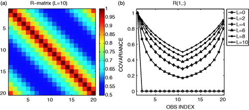A simple choice of a non-diagonal R is (9) where the observation-error variance is fixed at v = 1.0. L is the correlation strength parameter, so that larger values of L correspond to stronger observation-error correlations. In the limit of L = 0, R is diagonal. The R matrix is shown in Figure 1. Although we only show results for this case (Equation 9), other choices for R including negative correlations were tested, and they all yielded similar results.

Figure 1. Observation-error covariance R defined by Equation (9): (a) the full R matrix when L = 10; (b) the first column (or row) of the R matrix with various choices of L.

Correlated random numbers are generated using uncorrelated random numbers and the Cholesky decomposition of R. Let n(0, 1) denote a vector composed of 20 normally distributed uncorrelated random numbers drawn from N(0, 1). The vector of correlated random observation errors ε^o is given by (10) where R = CC^T is the Cholesky decomposition of R. The observations are then simulated by (11) where x^T is the nature state or ‘truth’. The analysis accuracy is measured by the root mean-square difference from the nature run, which we call root mean-square errors (RMSEs). The RMSE is averaged over the last 6 months of 1-year EnKF experiments to exclude the initial spin-up.

LKM09 developed an adaptive method to estimate observation-error variances and the covariance inflation parameter simultaneously. It uses the innovation statistics derived by Desroziers et al. 10 (12)

The bracket ⟨·⟩ indicates statistical expectation, usually obtained by averaging over many cases. LKM09 used this relationship and estimated observation-error variances successfully by assuming observations in each type of observation, e.g. wind and temperature, share the same error variance but without error correlations. In this study, we simply use the same Equation (12) to estimate the non-diagonal elements of R. Although we can apply the method to estimate each R for each group of observations, we assume the 20 observations in the present experiments are in the same group. In addition, we further assume that the error covariance is a function of the distance between observations in order to reduce the degrees of freedom of the R matrix. Namely, the 20 diagonal elements of the R matrix correspond to the zero distance, which is a single unknown. Similarly, the 20 elements adjacent to the diagonal correspond to the distance of two grid points, another single unknown, since the 20 observations are located at every other grid points. Overall, there are only 20 unknown elements needed to construct the full 20 × 20 R matrix. We have 20 observations or statistical samples to estimate the 20 unknowns at each assimilation step. The estimates are temporally smoothed by a simple weighted average with the prior estimate from the previous analysis cycle: (13)

Here, the subscripts indicate the assimilation time steps and is the estimate obtained from Equation (12) at time t. We use α = 0.03, i.e., we give 97% of the weight to the prior estimate. The initial (wrong) guess of the R matrix is a diagonal with a variance twice as large as the variance in the true R.

3. Results

Using a diagonal estimation of R from the original LKM09 method, the EnKF performs stably with observations with correlated errors (Figure 2, square marks). With various magnitudes of observation-error correlations varying from L = 0 (no correlation) to L = 10 (strong correlation), the RMSEs are below 0.4, less than a half of the observation-error standard deviation, and the RMSEs tend to decrease slightly with larger L. The estimated observation-error variance (i.e. diagonal values) is very close to 1.0, the true observation-error variance. As a result, using a fixed diagonal R with the true observation-error variance gives essentially the same analysis accuracy (not shown, but indistinguishable from the curve with square marks). When the diagonal R is inflated, for example to double the true observation-error variance, the analysis accuracy is degraded when the observation errors are correlated (Figure 2, triangle marks). The approach of using an inflated diagonal R is not appropriate to deal with observation-error correlations.

Figure 2. A 6-month average analysis RMSE for the cases of using true R (circle with thin dashed line), adaptively estimated non-diagonal R (cross), adaptively estimated diagonal R (square) and fixed diagonal R with twice the true variance (triangle). The abscissa indicates the observation-error correlation strength parameter L. The error bars indicate the standard deviation of temporal fluctuations. The two curves of true R and adaptively estimated non-diagonal R are nearly identical and on top of each other.

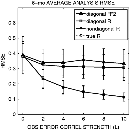
When the non-diagonal R is explicitly considered in data assimilation, the analysis accuracy is significantly improved as the observation-error correlations become more significant (Figure 2, cross and circle marks). Non-zero error correlations imply that the errors compared to the truth have similar patterns. Since we used the same number of observations to estimate such correlated errors, we were able to achieve a better analysis. In other words, the error correlation implies more information, and we can potentially extract more from observations by considering non-diagonal R explicitly in data assimilation.

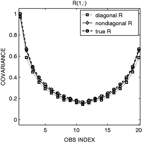
The straightforward extension of the LKM09 method for the non-diagonal R matrix performs properly and gives an analysis accuracy similar to that obtained using the true R (cross and circle marks in Figure 2). Several other choices for the true R matrix including negative correlations were tested, and they all gave essentially equivalent results, namely improving the analysis when estimating the error correlations. The 6-month average of the adaptively estimated R indicates very accurate estimation of the true R (cf. Figure 3 with Figure 1b). The time series of the adaptively estimated observation-error covariance indicates a certain level of noise (Figure 4), which largely depends on the choice of the time-smoothing parameter α in Equation (13). A larger α gives noisier time series due to sampling noise at each time, as shown by LKM09. Although a smaller α gives a smoother time series, it spins up more slowly. Using the Kalman filter update for Equation (13) as done by LKM09 provides faster spin-up, but the two approaches are essentially equivalent after the spin-up. The estimate is quite accurate after about 1-month spin-up; the initial guess of the R matrix (diagonal with twice as large observation-error variance) quickly approaches the true R values. Since the adaptively estimated R with some noise gave almost identical analysis accuracy as the true R (cross and circle marks in Figure 2), the sensitivity to the choice of α would not be significant; a smaller α would give smoother time series of estimated R, but the impact to the analysis accuracy would be small.

Figure 3. As Figure 1(b), but for the 6-month average of the adaptively estimated R. The error bars indicate the standard deviation of temporal fluctuations.

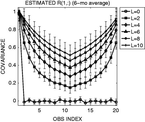
Figure 4. Time series of the adaptively estimated components of the full R matrix in the case of L = 10. Note: Thin dotted lines indicate the true covariance values. Each line type corresponds to the element R_ij whose grid distance d_ij between the ith and jth observations is as shown in legend.

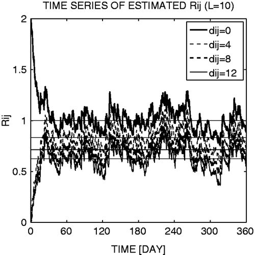
In real applications, it may be useful to first attempt to estimate the off-diagonal components of R without considering it in data assimilation. Namely, while using a diagonal R in EnKF assimilation, we can estimate a non-diagonal R in order to check whether the real observations have significant error correlations. The statistical relationship Equation (12) would be accurate if the full R matrix is considered in data assimilation and if the analysis is optimal. However, even when a diagonal R is used, we obtain fairly accurate estimate of non-diagonal R after spin-up (Figure 5). The results are encouraging, suggesting that it is possible to estimate a non-diagonal R of real observations without changing the current data assimilation system assuming a diagonal R.

Figure 5. First row (or column) of the true R matrix (dashed line with circles), adaptively estimated R matrix using non-diagonal R (solid line with diamonds) and diagonal R (dotted line with squares) in data assimilation.

4. Information content analysis

The results showed that the analysis was more accurate when observations had correlated errors. This implies more information available from observations with correlated errors. In information theory, entropy is a quantitative measure of information (e.g. 18). Stewart et al. 1 used entropy reduction (known as the Shannon information content) for numerically evaluating the information loss due to simplifying observation-error correlations. Entropy S is defined as a function of probability density function (PDF) p of probabilistic variable x: (14)

Larger entropy corresponds to less information. In data assimilation, observations are considered to be a probabilistic variable with multi-dimensional Gaussian PDF, i.e. the PDF of n observations is given by the n-dimensional normal distribution: (15) where indicates most probable values, which are usually observed values. Combining Equations (14) and (15), we obtain that the entropy of the observation PDF is given by (16) decreases if the diagonal terms are smaller and if the absolute values of the off-diagonal terms are larger. Since the logarithm function is monotonic, this implies that observations have more information if their error variances are smaller and if their error correlations are larger, which agrees with our results.

Although Equation (16) is considered to be the information of observations, it does not necessarily correspond to information available to the analysis through the data assimilation process. The following simple conceptual model highlights this point. Assume that we have two observations for a scalar variable, such as two thermometers in a small room. The observation operator H is given by (17)

A general non-diagonal observation-error covariance matrix R is (18) where the two observations have the error standard deviations σ₁ and σ₂, respectively, and there is an error correlation c. Assuming σ₁ = σ₂ = σ for simplicity, we obtain the analysis PDF of the Kalman filter analysis update which ensures the optimal use of observations: (19)

With a given background error P^f, the analysis error P^a is smaller when the two observations have negatively correlated errors (c < 0). Conversely, positive error correlations (c > 0) yield larger analysis errors than the case with uncorrelated errors. Therefore, even if observations have more information as given by the entropy in Equation (16), it may not ‘be available’ to reduce the analysis error in data assimilation. In summary, the available information of observations depends not only on R but also on H. Both R and H define the observing network, and their combination determines the available information in data assimilation.

In order to further elaborate the relation between the observing network and the available information, another simple conceptual model is considered. Let us assume two observations for a two-dimensional system. Assume the observing system is defined by (20) (21)

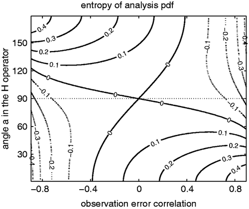
Here, information of observations is fixed at in order to purely focus on the available information. The observation-error correlations are given by and a is the angle between the two observations. Since θ is arbitrary due to isotropy, a and c are the two parameters that define the observing network. Without loss of generality, the background error covariance matrix is assumed to be the identity matrix: P^f = I. Since the analysis PDF of the Kalman filter update is the result of the optimal use of the observations, entropy of the analysis PDF is considered to be an indicator of the available information of the observations in data assimilation (Figure 6). The smaller the entropy, the more information is available from observations. When the observation errors are uncorrelated, the available information is maximum at a = 90°, i.e. the observation vectors are perpendicular. If the two observations observe a similar structure, the observation operator H is non-orthogonal, and less information is available in data assimilation. A typical example is satellite radiance observations whose channels have overlapping weighting function, so that the angles between different channels’ observation operators are not perpendicular. If a = 90°, i.e. H is orthogonal, the available information is minimum when the observation errors are uncorrelated. Namely, orthogonal observations carry more information when observation errors are correlated either negatively or positively. This agrees with the Lorenz model results in the previous section, in which only orthogonal H was considered, and both positively and negatively correlated errors improved the analysis accuracy. Uncorrelated conventional observations are a typical example of orthogonal H. The entropy of the analysis PDF (Figure 6) shows a general pattern of smaller values in the top-right and bottom-left corners, and of larger values in the top-left and bottom-right corners. The pattern corresponds to the previous one-dimensional case in the sense that the best combination is negatively (positively) correlated observations with positively (negatively) correlated errors. Therefore, the correlations in the observation operator have to be considered in addition to the observation-error correlations.

Figure 6. Entropy of analysis PDF, an indicator of available information of observations, as a function of the observation-error correlations (abscissa) and the angle between the two observations (ordinate). Note: The smaller the entropy, the more information is available from the observations.

5. Conclusions

Although at least some of the important observations in NWP have significantly correlated errors, the observation-error covariance matrix R is commonly assumed to be diagonal. This study aimed to investigate the impact of considering off-diagonal terms of R in data assimilation. One of the two important findings is that the error-correlated observations give a better analysis only when the non-diagonal R is explicitly considered in data assimilation. The results may appear to be against the intuitive notion that error-correlated observations may have less information. However, information theory tells us that off-diagonal terms of the error covariance matrix correspond to more, not less information. Moreover, the simple conceptual examples considered indicate that observations can provide more information to the analysis when the observation network has a favourable combination of the observation operator H and the observation-error covariance matrix R. Namely, more information is available from positively (negatively) correlated observations with negatively (positively) correlated errors. This can be further investigated by introducing various non-orthogonal H operators with the Lorenz model, which is a subject of future research.

The second main finding of this study is the successful and promising performance of the adaptive estimation of a non-diagonal R with EnKF. The method is a straightforward extension of the LKM09 method for adaptive estimation of a diagonal R to include off-diagonal components. The extended method provided fairly accurate estimate of observation-error correlations even with suboptimal data assimilation system using a diagonal R.

This study was carried out with only idealized low-order experiments and two conceptual experiments. It is important to further extend this study to estimating a non-diagonal R matrix of real observations, and to considering the non-diagonal R matrix in the local ensemble transform Kalman filter 17, with realistic NWP models. In real applications, a number of complications would arise, such as the inevitable presence of bias in both the observations and forecasts. Those biases would be spatially correlated and would naturally interfere with the estimate of the observation-error correlations. These possible complications should be identified and tackled in future studies.

Acknowledgements

The lead author (Takemasa Miyoshi) is grateful to Haroldo Fraga de Campos Velho of INPE (Brazilian National Institute for Space Research) for his kind invitation to the session IN22A ‘Inverse Problems in Geosciences’ at the AGU meeting in Brazil. We also thank Mark Buehner of the Environment Canada and Chris Snyder of the National Center for Atmospheric Research for insightful discussions. This study was supported by the Office of Naval Research grant N000141010149 under the National Oceanographic Partnership Program.

References

- Stewart, LM, Dance, SL, and Nichols, NK, 2008. Correlated observation errors in data assimilation, Int. J. Numer. Methods Fluids 56 (2008), pp. 1521–1527.
- Stewart, LM, 2009. Correlated observation errors in data assimilation. University of Reading, Reading: Ph.D. diss.; 2009, p. 195.
- Keeler, R, and Ellis, S, 2000. Observational error covariance matrices for radar data assimilation, Phys. Chem. Earth Part B 25 (2000), pp. 1277–1280.
- Bormann, N, Saarinen, S, Kelly, G, and Thepaut, J-N, 2003. The spatial structure of observation errors in atmospheric motion vectors from geostationary satellite data, Mon. Weather Rev. 131 (2003), pp. 706–718.
- Garand, L, Heilliette, S, and Buehner, M, 2007. Interchannel error correlation associated with AIRS radiance observations: Inference and impact in data assimilation, J. Appl. Meteorol. Climatol. 46 (2007), pp. 714–725.
- Bormann, N, and Bauer, P, 2010. Estimates of spatial and interchannel observation-error characteristics for current sounder radiances for numerical weather prediction. I: Methods and application to ATOVS data, Q. J. R. Meteorolog. Soc. 136 (2010), pp. 1036–1050.
- Bormann, N, Collard, A, and Bauer, P, 2010. Estimates of spatial and interchannel observation-error characteristics for current sounder radiances for numerical weather prediction. II: Application to AIRS and IASI data, Q. J. R. Meteorolog. Soc. 136 (2010), pp. 1051–1063.
- Li, H, Kalnay, E, and Miyoshi, T, 2009. Simultaneous estimation of covariance inflation and observation errors within an ensemble Kalman filter, Q. J. R. Meteorolog. Soc. 135 (2009), pp. 523–533.
- Daley, R, 1992. Estimating model-error covariances for application to atmospheric data assimilation, Mon. Weather Rev. 120 (1992), pp. 1735–1746.
- Desroziers, G, Berre, L, Chapnik, B, and Poli, P, 2005. Diagnosis of observation, background and analysis-error statistics in observation space, Q. J. R. Meteorolog. Soc. 131 (2005), pp. 3385–3396.
- Evensen, G, 1994. Sequential data assimilation with a nonlinear quasi-geostrophic model using Monte Carlo methods to forecast error statistics, J. Geophys. Res. 99 (C5) (1994), pp. 10143–10162.
- Evensen, G, 2003. The ensemble Kalman filter: Theoretical formulation and practical implementation, Ocean Dyn. 53 (2003), pp. 343–367.
- Anderson, JL, and Anderson, SL, 1999. A Monte Carlo implementation of the nonlinear filtering problem to produce ensemble assimilations and forecasts, Mon. Weather Rev. 127 (1999), pp. 2741–2758.
- Lorenz, E, , Predictability: A Problem Partly Solved, Proceedings of the ECMWF Seminar on Predictability, Vol. 1, Reading, UK, 1996.
- Lorenz, E, and Emanuel, K, 1998. Optimal sites for supplementary weather observations: Simulation with a small model, J. Atmos. Sci. 55 (1998), pp. 399–414.
- Whitaker, JS, and Hamill, TM, 2002. Ensemble data assimilation without perturbed observations, Mon. Weather Rev. 130 (2002), pp. 1913–1924.
- Hunt, BR, Kostelich, EJ, and Szunyogh, I, 2007. Efficient data assimilation for spatiotemporal chaos: A local ensemble transform Kalman Filter, Phys. Nonlinear Phenom. 230 (2007), pp. 112–126.
- Rodgers, CD, 2000. Inverse Methods for Atmospheric Sounding: Theory and Practice. Vol. 2. Singapore: World Scientific; 2000. p. 256.