Calibrating an hydrological model by an evolutionary strategy for multi-objective optimization

Abstract

Hydrologic models simulate the river flow from the contributing basin for a given river. For the simulation process, the integration domain is discretized into computational cells. The inputs for such models are precipitation ratio and the initial flow. There are many parameters to be determined for an operational model, including the type of soil (porosity field, water flux between the bottom of the river and the water layer, among others). The process to identify the best numerical values for such parameters is the calibration procedure, belonging to the class of inverse problems for parameter determination. However, there is no unique set of parameters for representing the hydrology cycle. A multi-objective approach is employed to address the problem. The Pareto set is calculated for the IPH2 model by an epidemic genetic algorithm.

Keywords:

• parameter estimation
• hydrological model
• epidemic genetic algorithm
• multi-objective optimization
• Pareto set

1. Introduction

Several processes from the hydrological cycle acting in the watershed can be represented by simplified mathematical models to simulate the transformation of rainfall into runoff: rainfall–runoff models. From these models, it is possible to understand better hydrological phenomena, description of hydrological scenario, appropriate sizing, for providing data when there is no observational data, analysis on the effects coming from the change of the land use and prediction of hydrological variables (e.g. river flow) in real time 1.

Hydrological models of the rainfall–runoff type consist of parameters to characterize the system, some of them represent abstractions of reality and, due to this, they cannot be measured 1. Such parameters must be adjusted, taking into account the existing hydrological information in the basin. This process is known as calibration. However, there are many simplifications in the model with impact on the representativeness of the parameters; in addition, there are also uncertainties in the data. Therefore, the calibration process could not be, in practice, a unique set of parameters able to represent the hydrological processes. Indeed, calibration is a mathematical problem of many (maybe infinite) solutions, all of them equally possible, with some of them unable to represent the reality of the phenomenon, or even the expected values. On the other hand, solutions technically acceptable may not be possible to distinguish as more acceptable or better.

The manual calibration (trial-and-error) is one of the pioneering techniques of calibration. It consists in procedure with interaction, in which the user changes the values of the model parameters for each trial, and compares the results from the model with the measured results, until the results reach a set of parameters for which the model results are most appropriate for the simulated process. The comparison of each attempt can be made visually (e.g. using hydrograph or by using objective functions, computing some kind of error measure (norm) between the flow values calculated by the model and the values of the observed flow. Such functions aimed to evaluate the quality of adjustment, some norms more sensitive to maximum flows, and other norms more appropriate for evaluating the adjustment to the minimum flows. Despite its robustness and simplicity, the manual calibration depends on the ability of the user; in addition to understanding the model, the analyst must have the ability to find a solution by trial, even if multiple objectives are considered. The absence of a measurable criterion for comparison, and the use of subjective criteria, leading to different set of parameters for different users, can be identified as major deficiencies of the manual calibration.

The calibration process becomes faster and more efficient by using automatic calibration techniques based on the intensive use of computers. In these techniques, the basic procedures for setting the parameters in rainfall–runoff models consider the following: one or more objective functions, an optimization algorithm and a stopping criterion. Therefore, the calibration of hydrological model parameters becomes an optimization problem of a single function (mono-objective calibration) or more than one function (multi-objective calibration).

Mono-objective calibration considers a single measure of performance among the various possible (usually based on the error between the observed and the flow measures), obtaining as a result a unique set of parameters to optimize the performance of the comparison (data from observations and the model).

In multi-objective calibration, the goal is to optimize more than one performance measure, simultaneously, resulting in multiple sets of parameters that will provide a set of optimal solutions (Pareto set). It is expected that from this set of optimal solutions, a desired response to the model fit can be obtained.

Different multi-objective optimization algorithms have been developed. Evolutionary algorithms are one of these approaches, and they have received more attention in the past four decades.

This article presents an epidemic genetic algorithm (EGA) 2,3 for multi-objective calibration of the hydrological model IPH2 1. Our algorithm could be considered as a variant of the evolutionary algorithm MOCOM-UA (Complex multi-objective Evolution, University of Arizona) 4, which combines the techniques of evolutionary algorithms with the simplex algorithm of Nelder and Mead 5. The MOCOM-UA algorithm is already been used for the calibration of the IPH2 model.

2. The multi-objective calibration problem

2.1. Formulation

In a hydrological rainfall–runoff model, the estimated flow depends, at each time interval , on the values of precipitation , evaporation and the parameter set , that is: (1) where represents the hydrological model. The difference between simulated values and observed data (these differences represent the errors in estimating the model at each time interval) is defined by: (2)

The performance measure of the hydrological model can be done in different ways by means of functions . Such functions are called objective functions. Several types of objective functions can be used in the calibration of hydrologic rainfall–runoff models. Some give greater weight to the errors of maximum flows (floods) and others assess better the fit to the low flows (dry period). In the following equations, we have four examples of objective functions: (3) (4) (5) (6)

The multi-objective calibration of a hydrological model can be described as a multi-objective optimization problem with the following general formulation: (7) where are the different objective functions to be simultaneously minimized, are the constraints of the problem and is the vector of parameters of an n-dimensional parameter space . The evaluation function maps the space of parameters (decision variables) in the objective space .

2.2. Pareto set

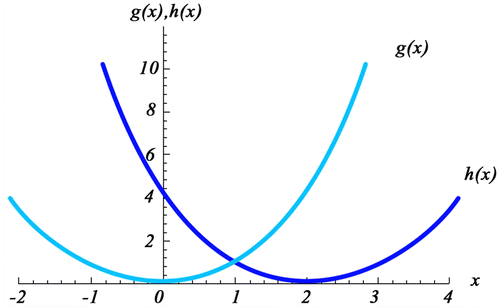
The main characteristic of a multi-objective optimization problem is that the solution will not, in general, be unique. Often, there are several solutions such that, moving from one solution to another, causes the improvement of one objective function while resulting in a deterioration in the value of at least another objective function. Therefore, it is necessary to identify, among the solutions, those which are efficient for solving the problem. Figure 1 illustrates the situation described above, for a simple problem where two objective functions and are to be minimized with respect to one real parameter 6. The solutions of the problem consist of all points in the interval . For , is smaller than . On the other hand, for , is larger than . Because each function is its own entity, it is not possible to determine, objectively, among such solutions, which one is the best. Such solutions are called Pareto, non-dominated or efficient solutions 4.

Figure 1. Functions g(x) and h(x) of a multi-objective problem.

The following formulation 4 establishes the division of the feasible parameter space into two parts: one of the non-dominated solutions (Pareto set) and another of the dominated solutions. By definition, any solution belonging to the Pareto set must satisfy the following properties:

1.	is strictly less than , for all solutions not contained in the Pareto set;
2.	there is no solution in the Pareto set, such that is strictly less than .

The space of feasible solutions is then partitioned into two sets, one of the ‘good’ solutions (Pareto solutions) and another of the ‘bad’ solutions, and it is not possible to distinguish, among the ‘good’ solutions, which is the best one.

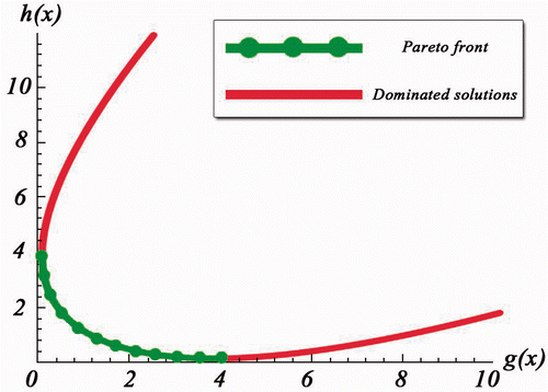
The set of non-dominated solutions is, therefore, the goal of multi-objective calibration. The mapping of this set in objective space forms a surface known as Pareto front. Figure 2 shows the Pareto front for the functions g and h from the previous example. Moving along the Pareto front, an improvement in one of the objective function is accompanied by a worsening in the other function. In this case, with only two objective functions, it was easy to identify the Pareto front. For more complex problems, however, a graphical analysis cannot be made, and it is essential to use computational techniques to obtain an approximation of the Pareto front. In the calibration of a hydrological model, it is desirable an approach to allow the identification the largest number of non-dominated solutions, in order to obtain a good representation of the modelled process.

Figure 2. Objective space Z = (g, h).

Several techniques have been proposed to generate good approximations of the Pareto front. Some of them are based on introducing different weights (penalties) for each partial objective function, and reducing the problem to a mono-objective optimization problem 7,8. Some methods, usually interactive, seek to generate only a subset of Pareto set of previous interest. Others require choosing a solution among several alternatives.

More efficient techniques were presented by Yapo et al. 4 and Erickson et al. 9, using the concept of ‘Pareto's hierarchy’ or Pareto's ranking, allowing to find several points in the Pareto front in only one optimization procedure. The algorithm developed by Yapo et al. 4, called MOCOM-UA, is based on the techniques of evolutionary algorithms and the downhill simplex method 5.

2.3. Genetic algorithms

A genetic algorithm (GA) 10 is a meta-heuristic inspired from Darwin's theory of evolution. It simulates the process of natural selection and survival of the fittest individuals.

In an optimization problem, a GA tries to find a good solution, from an initial random population, consisting of potential solutions to the problem, and manipulating these solutions by genetic operators. These operators use the existing solutions to produce new solutions, expected to be better than previous solutions, for responding the evolution pressure (the fitness or objective function). For each individual from the population, a scalar fitness value is determined, which represents a numerical measure of individual ability to give an answer to the problem. One idea is to select the solutions with better fitness (elitist strategy), and apply genetic operators on them, in order to generate the next generation with better individuals, that is, better solutions to the problem.

The basic entities of a GA have their name associated with terms from the biology. The set of candidate solutions of the problem is called population, such elements being called individuals or chromosomes. Each individual has a basic unit, called gene, which describes a certain variable of the problem. Each iteration is called generation. The operations used on individuals of the population to produce better solutions are called genetic operators.

Representation or coding of variables in a GA can be binary, or integer, or real. The generation of the population can be done randomly or using a heuristic. The evaluation of the population is made using one or more fitness functions to evaluate the quality of solutions (for multi-objective optimization, the objective functions are used). The selection of individuals is a mechanism used to preserve good characteristics of individuals. It can be done by ranking, by a tournament, etc. The basic genetic operators are: selection, crossover and mutation, used to generate the fittest individuals, that is, better solutions to the problem.

The crossover operator makes changes or combinations of sequences of information between individuals of the population, generating new individuals with inherit characteristics of the previous individuals. It tries to be quite similar to chromosomal union to form new combinations of genes. In order to maintain the diversity of the solutions, individuals with very similar characteristics, possibly generated by the crossover operator, should be eliminated. The techniques of drafting crossover operators take in account the genetic representation with which one works. For example, the following techniques can be mentioned: one-point crossover, multiple-point crossover and uniform crossover.

The mutation operator is applied to randomly change the value of one or more genes of a chromosome. Contrary to the crossover operator, it does not increase the population numerically, it only modifies existing individuals transforming them into different other individuals. If an individual resulting from the mutation operator already exists, it is discarded. The mutation operator allows a greater genetic diversity and a further exploration of the search space and prevents the algorithm to be stationed at local minima.

In order to increase the speed of the algorithm convergence, the best solutions found in a particular generation are preserved for using in future generations, leading to the elitism. One of the most important aspects in the structuring of a GA is the control of its parameters: population size, crossover rate and mutation rate.

2.3.1. Epidemic operator

In addition to the genetic operators mentioned above, a new operator can be considered, and it was used in the GA presented here. It is the epidemic operator, or simply epidemic 2,3. This operator is activated when, after a certain number of generations, there is no improvement in the population. It can also be used to prevent or solve a problem of premature convergence. This operator simulates the occurrence of an epidemic on the population, decimating the less fit individuals, so that those with better skills are preserved. Eliminated individuals are replaced by new elements, generated by the same process of generating the population and the evolution process is restarted. A comparison of stochastic strategies was carried out by Cuco et al. 11, and they have shown the effectiveness of the epidemic GA.

3. A multi-objective GA for calibrating of hydrological model

The EGA will be presented here. It is a variation of the evolutionary algorithm MOCOM-UA – mentioned earlier. Its steps are described below, and the first five steps are identical to the MOCOM:

1.	Initially, the minimum and maximum values of the k unknown parameters are established, thereby defining a feasible region for the parameters.
2.	Using a uniform distribution, sets of the model parameters inside the feasible region are generated. Each set of parameters is a point in the parameter space, whose coordinates are the values of the parameters. Each one of these points is an individual of the population.
3.	The points of the population are evaluated with the nf objective functions, generating a matrix of results .
4.	The following Pareto's ranking 10 is applied: The non-dominated individuals in the population are identified and they are assigned the rank 1. These individuals are temporarily removed from the population. The non-dominated individuals identified in the remaining population are assigned the rank 2. These individuals are temporarily removed from the population. The process is repeated until every point has been assigned a rank. The worst individuals of the population are those individuals that are most distant from the Pareto front, having the highest value of rank, . In this way, rank values are assigned to each point i of the population, ranging from 1 to , where . The best individuals of the initial population (non-dominated) have a rank equal to 1, and the worst individuals have a rank equal to . With this sorting, in the objective space, fronts of dominance are created and they indicate the level of dominance of one solution over others.
5.	Creating complex sets: Each individual with a rank equal to will result in a set called complex. Complex consists of individuals, where one is an individual of rank , and the remaining (number of model parameters) are randomly selected from among individuals in the population that have no rank equal to , using the following equation of probability associated to each point :

The probability of an individual to be selected depends on its rank being favoured those with lower rank (the best). Different complex sets may have elements in common.

1.	Here, the evolution of the complex sets is computed to enhance the convergence of the population to the Pareto front. In this algorithm, a genetic evolution is applied to each complex. Given complex, genetic operators of mutation and crossover are applied to its individuals, generating new elements (offprints) until, considered the ranking done in the complex, the individual with the lowest rank has a rank lower than the maximum rank in the complex before operations. Some parameters were considered. A parameter to identify the maximum number of attempts of generations for each complex until an individual is better than the individual with maximum rank. Another parameter is also considered for activating the epidemic operator, applied to all individuals in the population whose rank values are greater than or equal to a certain value (which is also a parameter). The latter action can be translated as: all individuals whose rank values are greater or equal than a preset value are eliminated from the population and other individuals are generated, in the same way that the initial population, and go back to step 3. The application of epidemics has also been limited to a maximum number of iterations.
2.	After the evolution of all complex sets, the individuals are returned to the population.
3.	Test of convergence. The stopping criterion for the algorithm finishes the process when all individuals of the population are non-dominated, that is , or when a maximum number of interactions is achieved.

4. Calibration of the IPH2 model

4.1. A brief description of the IPH2 model

The hydrological model IPH2 is a rainfall–runoff model in which the hydrological processes are represented by variables concentrated in space and the basin is represented by a mean precipitation 1. Therefore, it is suitable for small basins, where the spatial distribution of parameters and variables does not affect the results of its simulations. It is composed of three algorithms: one to compute the loss by evaporation and interception, other for calculating the separation of flow and the last one for the propagation of surface runoff and groundwater runoff.

The algorithm of losses by evaporation and interception takes a single parameter, , which describes the maximum capacity of storage in a reservoir of losses. In the flow separation algorithm, there are three parameters from the Horton equation: the parameters and , representing the initial and minimal capacities of infiltration in the soil, respectively, and the parameter H, the variation of soil infiltration capacity. The parameter H is defined by de equation: , where is an empirical parameter related to the soil type, characterizing the exponential decay of the infiltration curve. The spread of runoff is made with the method of Clark, using concentration–time parameters that can be kept fixed or calibrated, depending on the availability of physical characteristics of the basin. Using the simple linear reservoir theory to consider the effect of storage in the basin, there is the parameter , which represents the delay time of the runoff. The percentage of impermeable area of the basin should be set. For the spread of groundwater flow, it is also used a simple linear reservoir model with the parameter , which represents the average time to empty the reservoir of underground runoff 12. For the simulation of a continuing series of long period, it was introduced a parameter , only used in the simulation of the separation of the flow for the event where the infiltration capacity exceeds precipitation 12. It represents the direct flow of impermeable areas. For simulating the process, in addition to the seven parameters mentioned before, the basin area and the input variables for the model (precipitation and evaporation) should be informed 12.

4.2. Some calibration results with IPH2 model

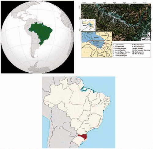
Calibration tests of the IPH2 model were performed with EGA and MOCOM strategies. The direct model was run with values of the seven parameters of the IPH2 model, and actual data of precipitation and evaporation (301 records) from the Canoas river basin, Santa Catarina (Brazil), with an area of 989 km² (Figure 3). The data period was 11 March 1983–5 January 1984, with diary data.

Figure 3. Canoas river basin: local map.

A series of flows was then obtained. For emulating observations a 5% of noise was added to the output values from the IPH2 model. The synthetic observations of flow were used for the calibration procedure. The values assigned to seven parameters to generate synthetic series were 13: , , , , , and .

The objective functions considered in the tests were the following: F₁ (standard deviation of flows) and F₂ (standard deviation of inverse flows), described in Equations (3) and (4), respectively. The maximum and minimum limits for the parameters of the IPH2 model are presented in Table 1.

Table 1. Maximum and minimum values to the parameters of the IPH2 model.

Parameter	Unit	Minimum value	Maximum value
		10.00	300.00
		0.10	10.00
	–	0.01	0.999
		0.01	10.00
		10.00	500.00
		0.00	9.00
	–	0.01	20.00

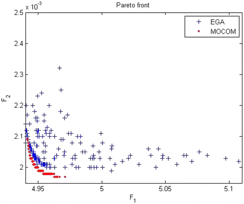
The size of the initial population is the only parameter for the MOCOM algorithm. For the EGA algorithm, beyond the size of population, other parameters are needed, as mentioned. Tests were performed with a population size , which is considered as satisfactory for the desired calibration using the MOCOM 13. For this population size, there was a difficulty for the convergence of the EGA to compute the Pareto front, although the values obtained for the objective functions were very close to those obtained by using the MOCOM. A very large number of interactions occurred without obtaining a population in which all individuals were non-dominated.

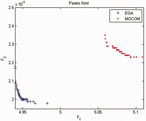
Figure 4 shows the Pareto front in the objective space, for the tests of calibration of the IPH2 model using the two algorithms, EGA and MOCOM, with a population size in both. Tests considered the maximum number of generations equal to 1000 for the EGA. From the figure, the EGA stopped before reaching a population in which all individuals were non-dominated. However, the values of objective functions are quite similar to the parameter setting with the MOCOM.

Figure 4. Objective space: calibration with EGA and MOCOM, with population (ns) equal 200.

Better results with the EGA were obtained when considering the population size . Several tests were carried out to establish the following set of parameters for the EGA:

•	Maximum number of iterations: MAX_ITER = 5000.
•	Rate of mutation: TAX_MUT = 0.03.
•	Maximum of attempts of evolution of complex: MAX_GER = 100.
•	Activation rate of the epidemic (percentage of complex without evolution at which the epidemic is on): TAE = 0.70.
•	Epidemic rate (indicates in which individuals the epidemic will be applied): individuals with a rank higher or equal to will be eliminated.
•	How long epidemics will be applied: until the number of iterations to reach half the value of the parameter MAX_ITER.

Figure 5 shows the calibration results of the IPH2 model, using the two algorithms, MOCOM and EGA (with the EGA parameters mentioned above), considering a population size for both schemes. The better solution to the Pareto front is that closer to the origin.

Figure 5. Objective space: calibration with EGA and MOCOM, with population (ns) equal 50.

The two strategies, MOCOM and EGA have shown quite satisfactory to retrieve good values for the parameters of the IPH2 model. Table 2 presents the maximum and minimum values of each of the parameters obtained with the automatic calibration for the IPH2 model, with the two strategies: EGA and MOCOM. Several simulations were considered, with a population size , and the parameters of EGA with the adjustments listed above. For both strategies, the range of variation of the parameters was relatively narrow. This is a good indication on the validity of the hydrological model. The values for the parameter obtained by EGA are very close to the upper set limit, indicating the necessity to expand this limit.

Table 2. Minimum and maximum values of the parameters of the IPH2 model, in a multi-objective calibration, using EGA and MOCOM.

Parameter	Unit	Range of variation
		MOCOM		EGA
		Minimum	Maximum	Minimum	Maximum
		11.72	23.45	22.60	27.04
		2.64	3.05	2.87	3.08
	–	0.028	0.077	0.035	0.40
		5.61	5.68	5.60	5.73
		35.89	47.53	35.76	43.29
		0.01	1.53	0.44	0.86
	–	4.89	9.94	17.04	20.00

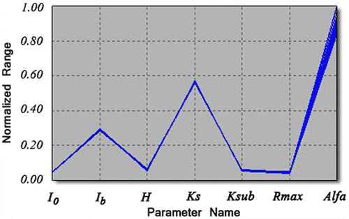
Figure 6 shows a graph for all the parameters with non-dominated individuals (Pareto solutions) obtained with the EGA calibration strategy. The parameter presented the largest range.

Figure 6. Parameter space.

5. Conclusions

Computers developed to be faster and much more powerful enabling the emergence and improvement of various computational techniques to solve problems of parameter calibration, common in modelling a given phenomenon. In the case of hydrological models, multi-objective calibration has gained more space, since it allows a better evaluation of the uncertainties, the imperfections of the model and the representativeness of parameters.

This article presented an EGA as a possible alternative for the calibration of hydrologic models, and it has been tested for the calibration of the hydrological model IPH2, a model already well established for small basins, efficient in the simulation of processes and applied for several Brazilian basins using the MOCOM algorithm.

The results presented here are preliminary and were produced from tests based on synthetic observations of flows. The EGA algorithm was efficient in recovering the correct values of the parameters, and for finding a good approximation of the Pareto front. Some comparisons between the results obtained with the EGA and those obtained with the MOCOM algorithm were presented. The results obtained by using the EGA algorithm are promising, placing it as a good alternative to automatic calibration in others more sophisticated hydrological models, in which much more variables of the hydrological cycle, such as evapotranspiration and the level of underground water, may be taken into account, and in applications where several models are coupled.

Acknowledgements

The authors thank Profs Walter Collischon and Juan Martin Bravo, both from the Institute of Hydraulic Research of Federal University of Rio Grande do Sul, Brazil, who has provided full support for the tests with the IPH2 model. Professor Juan provided the program WIN_IPH2 12, which couples the hydrologic model IPH2 and the calibration algorithm MOCOM, and the data for the basin that were used in calibration tests. H.F. Campos Velho also thanks the CNPq, Brazilian agency for research support.

References

- Tucci, CEM, 1998. Modelos hidrológicos. Porto Alegre: ABRH Editora da UFRGS; 1998.
- Medeiros, FLL, , Hybrid genetic algorithm as a search scheme of steady state of dynamical systems, M.Sc. thesis, Instituto Nacional de Pesquisas Espaciais (INPE), São José dos Campos (SP), Brazil, 2002.
- Chiwiacowsky, L, and Campos Velho, HF, 2003. Different approaches for the solution of a backward heat conduction problem, Inv. Probl. Eng. 11 (6) (2003), pp. 471–494.
- Yapo, PO, Gupta, HV, and Sorooshian, S, 1998. Multi-objective global optimization for hydrological models, J. Hydrol. 204 (1998), pp. 83–97.
- Nelder, JA, and Mead, R, 1965. A simplex method for function minimization, Comput. J. 7 (1965), pp. 308–313.
- Schaffer, JD, , Multiple objective optimization with vector evaluated genetic algorithms, Ph.D. thesis, Vanderbilt University, Nashville, TN, 1984.
- Zadeh, LA, 1963. Optimality and non-scalar valued performance criteria, IEEE Trans. 8 (1) (1963), pp. 59–60.
- Goicoechea, A, Hasen, DR, and Dukstein, L, 1982. Multi-objective Decision Analysis With Engineering and Business Applications. New York: John Wiley; 1982.
- Erickson, M, Mayer, A, and Horn, J, 2002. Multi-objective optimal design of groundwater remediation systems: Application of the niched Pareto Genetic Algorithm (NPGA), Adv. Water Res. 25 (2002), pp. 51–65.
- Goldberg, DE, 1989. Genetic Algorithms in Search, Optimization and Machine learning. New York: Addison–Wesley; 1989.
- Cuco, APC, Silva Neto, AJ, Campos Velho, HF, and Souza, FL, 2009. Solution of an inverse adsorption problem with an epidemic genetic algorithm and the generalized extremal optimization algorithm, Inverse Probl. Sci. Eng. 17 (13) (2009), pp. 289–302.
- Bravo, JM, Allasia, DG, Collischom, W, Tassi, R, Meller, A, and Tucci, CM, , Avaliação visual e numérica da calibração do modelo IPH II com fins educacionais, Anais do XVII Simpósio Brasileiro de Recursos Hídricos, São Paulo (SP), Brazil, 2007.
- Bravo, JM, Collischon, W, and Tucci, CEM, 2009. Verificação de eficiência de um algoritmo evolucionário multiobjectivo na calibração automática do modelo hidrológico IPH II, Revista Brasileira de Recursos Hídricos-RBRH. 14 (2009), pp. 37–60, Porto Alegre, RS.