Firefly optimization to determine the precipitation field on South America

Abstract

A model simulation of an intense rainfall associated with a case of South Atlantic Convergence Zone that occurred during 21–24 February 2004 using the Brazilian developments on the Regional Atmospheric Modelling System was performed. The convective parameterization scheme of Grell and Dévényi was used to represent clouds of the sub-grid scale and their interaction with the large-scale environment. This method is a convective parameterization that can make use of a large variety of approaches previously introduced in earlier formulations, considering an ensemble of several hypotheses and closures. The rainfall was evaluated by six experiments, using different choices of rainfall parameterizations, providing six different simulated responses for the rainfall field. The sixth experiment ran with an average among five closures (ensemble mean). The purpose of this study was to generate a set of weights to compute a best combination of the ensemble members. This inverse problem of parameter estimation is solved as an optimization problem. The objective function was computed with the quadratic difference between five simulated precipitation fields and observation. The precipitation field estimated by the Tropical Rainfall Measuring Mission satellite was used as observed data. Weights were obtained using the firefly optimization algorithm and it was included in the cumulus parameterization code to simulate precipitation. The results indicated the better skill of the model with the new methodology compared with the old ensemble mean calculation.

Keywords:

• cumulus representation
• precipitation
• BRAMS
• firefly optimization
• inverse problems

1. Introduction

Several processes from the hydrological cycle acting in the watershed can be represented by simplified mathematical models to simulate the transformation of rainfall into runoff: rainfall–runoff models. From these models, it is possible to understand better hydrological phenomena, description of hydrological scenario, appropriate sizing, provide data when there is no observational data, analyse on the effects coming from the change of land use and predict hydrological variables (river flow, for example) on real time 1.

Precipitation is one of the most relevant meteorological variables related to weather and climate. Several sectors of society and the economy demand knowledge of the precipitation distribution on space and time, for example, the management and monitoring of water resources, a key issue for the agriculture and/or energy production, for the countries like Brazil, as well as the prevention or mitigation of the effects from the severe weather: action or control of deep dry seasons, or flood condition. The quantitative treatment for the precipitation prediction is a challenge because there is no unique parameterization with good performance for all regions in the world 2.

The precipitation results from a complex process of energy and mass (moisture) transfer between the surface and the atmosphere. Such processes are developed on very small time and space scales, with the order of minutes and centimetres. The water vapour convective process determines the cloud development (it could be small, medium, or high). The precipitation is the final step for long and complex thermo-dynamical exchanges.

Clouds of all scales and meso-scale precipitating systems have a prominent rule for the general circulation of the atmosphere. They impact the climate system on radiation balance, changing the temperature, pressure and velocity fields 3. The clouds are important for the natural greenhouse effect, essential to the human beings, and maintain a comfortable average temperature for the planet. The study of the dynamics and the energy changes associated to the clouds, mainly the deep convection, is very important for a better understanding of atmospheric systems of large scale 4.

During the past decades, a remarkable effort is focused on representing the clouds and their process on the environment in the numerical models. However, an appropriated representation would be obtained using a horizontal resolution ranging from 102 up to 103 m. For this level of resolution, it is very expensive from the computational point of view 4), even for today. Therefore, an important issue for numerical weather prediction, for regional and global models, in numerical simulation of phenomena, such as fronts and cyclones, is to estimate the physical effects of the cumulus convection on the resolvable scales of the movement by developing quantitative relationships between the cloud effects and the known parameter of the larger-scale model 4. For relating the sub-grid effects from the clouds in the resolved movement scales by the model is known as cumulus parameterization.

Cloud parameterization is still considered an open problem, even if there are several schemes for this kind of cloud parameterization 5–10, because a correct prediction is a persistent challenge.

Grell and Devényi 10, hereafter cited as GD, have introduced a flux mass formalism based on multi-model ensemble. In this approach, the net effect from the feedback cycle (environment–cloud) is obtained from the statistical method to compute the optimal values to the set of parameters to express the precipitation in the model. The GD parameterization can be applied using different closure schemes together. The ensemble of parameterizations is to improve the prediction skill. The members of the ensemble are obtained from perturbations in the function of the convection triggering.

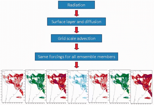
The ensemble set from the GD scheme implanted in the BRAMS (Brazilian Regional Atmospheric Modelling System – see: Freitas et al. 11) is constituted by the parameterizations from Grell 9, Arakawa and Schubert 6, Kain and Fritsch 12, low-level omega 13 and moisture convergence 14, hereafter cited as GR, AS, KF, LO, MC, respectively. Figure 1 shows a simplified description from the GD parameterization. For each time-step in the computer model, some fields and parameters are collected (radiation, surface flux and turbulent diffusion in the planetary boundary layer – PBL), and the total forcing term is computed for all grid points and applied to the ensemble members. Total forcing is a summation of the sub-grid scale forcing (radiation, surface flux and turbulent flow in the PBL) and the large-scale terms (advection on the grid scale). For each different parameterization, there is a threshold (a trigger function) that determines the generation of precipitation, and if this is true, the mass flux and the precipitation are calculated according to parameterization from the ensemble members.

Figure 1. Flowchart for representing cumulus parameterization by multi-model ensemble of Grell and Dévényi 10.

The final result is a set of precipitation predictions. There are several ways to combine such predictions, in order to get a numerical representation for the forecasting for precipitation and the atmospheric ratios for the heat and moisture fluxes. For the current BRAMS version, there are some options to be defined by the user:

1.	Defining a specific parameterization: , mass flux for a given ensemble member.
2.	Ensemble average (ENS): .

The ensemble technique has presented good performance 15,16. The goal of this article is to improve the results of the multi-model ensemble approach. The idea is to identify automatically the contribution of each member in the ensemble. This is a type of parameter estimation inverse problem 17.

There are many applications of inverse methodology in meteorology. An important inverse problem is to retrieve the temperature and moisture atmospheric profiles from satellite data 18–24. Other examples of inverse problem in meteorology are: identification of glacier instability 25, data assimilation 26,27, a modern use for determining the source of pollutant emission 28 and the bio-geochemical cycle for the atmospheric gases 29–33.

Inverse problems belong to the class of ill-posed problems 34. There are several methods to compute an inverse solution 35,36. Regularization technique becomes the original inverse problem in a well-posed one, where a constraint is applied to find a subset of appropriate solutions. In this study, the inverse problem is formulated as an optimized problem. The optimization problem is solved by a firefly stochastic scheme 37, and the objective function defined by the square difference between the predicted precipitation field and the precipitation observed. The experimental data to the rain simulation on South America is provided by Tropical Rainfall Measuring Mission (TRMM) satellite data.

First, the methodology is tested on two synthetic experimental data sets. Second, the approach is employed to simulate an event of intense rainfall on South America on 21 February 2004. This intense rainy period was associated with the South Atlantic Convergence Zone (SACZ, or ZCAS for the acronym in Portuguese: Zona de Convergência do Atlântico Sul), during 21 up to 24 February 2004.

2. Field precipitation identification

As already mentioned, the inverse solution is obtained by solving an optimization problem. The smoothest precipitation field is a constraint used. The constraint is added to the objective function with the help of a Lagrange multiplier: (1) where J(W) is the objective function, P^W the computed precipitation field, w_i the element of the weight vector W (here, N_w = 5), Λ the regularization operator and η the regularization parameter. The Tikhonov regularization of zeroth order was used, and it is given by (2) where the Frobenius norm was adopted to evaluate the measuring of the smoothness of the precipitation on the region. There are several methods to estimate the regularization parameter, among them the Morosov's discrepancy principle, L-curve and cross-validation are some. Here, the value η = 0.1 was determined by numerical experimentation.

2.1. Forward problem

The BRAMS model, version 4.311, was employed to simulate 1 day of intense precipitation on South America during a SACZ event. The BRAMS was integrated for 48 h, from 19 February 2004 at 12:00 UTC, with new initialization at every 24 h, until the end of the day 24 February-2004. The horizontal resolution was 25 km, with 38 levels for the vertical coordinate, where the first level placed at 100 m over the surface, and for moisture initialization, the heterogeneous soil representation was used and updated 16,38. The turbulence is modelled by Mellor-Yamada's 39 scheme, and the vegetation covering is represented by the Olson Global Ecosystem (OGE) 40 – outside Brazil and PROVEG data within Brazil – see 41, 42. The surface model is the Land Ecosystem-Atmosphere Feedback version 3 (LEAF-3) 43,44. BRAMS uses parameterizations for microphysics (45,46) and the convective parameterization employed was the GD-2002, where the ensemble closure was constituted by GR, LO, MC, KF and AS.

For the initial and boundary conditions, the analysis from the general circulation model (MCGA) from the CPTEC–INPE (CPTEC, Center for Weather Prediction and Climate Study; INPE, National Institute for Space Research), with resolution T126L28, where T126 represents the rhomboidal truncated with 126 terms in the spherical harmonic expansion and L28 the 28 vertical levels in the MCGA–CPTEC model. The analysed variables were the convective precipitation and the ascending and descending mass fluxes.

The BRAMS model was run with five parameterization schemes separately, obtaining five different simulations for the day, 21 February. Each simulation is a member of the forward problem.

2.2. Experiments with synthetic observation

Numerical experiments were designed to evaluate the methodology. In the experiments, the synthetic observed precipitations were obtained from combining five simulations for each parameterization. Table 1 presents the indexed weight for each cumulus parameterization. The weights were chosen from a previous qualitative analysis 47. From such analysis, the results indicated that parameterizations AS, GR and KF had a better agreement with the precipitation field measured by the TRMM data on 21 February 2004. Therefore, these parameterizations will be represented by heavier weights having a greater contribution for the ensemble.

Table 1. Weights for the synthetic precipitation field.

Parameterizations	Weight
WAS	0.25
WGR	0.35
WKF	0.20
WMC	0.15
WLO	0.05
Summation	1.00

Therefore, the precipitation field is given by (weights from Table 1): (3) where P_k (k  = AS, GR, KF, LO or MC) are the precipitation fields computed from the parameterizations. In order to have a better representation for the experimental data, a noise is added to the precipitation field (3): (4) where σ = 0.02 is the level of the noise and μ a random value with Gaussian distribution. Indeed, the data from the satellite TRMM presents errors on space and time over South America 48,49.

2.3. Experiment with real observations

In the second experiment, the simulations were also carried out for the day 21 February 2004. The objective function P(W) is for every horizontal grid point in the BRAMS model with the vector W(x, y). The observation field P_O was obtained from the TRMM satellite data (5)

The set of weights distributed on space was included in the computer model using an interpolation of the nearest neighbour 50 (http://en.wikipedia.org/wiki/Nearest-neighbor_interpolation). The interpolation procedure is designed to allow any defined space resolution. Each weight was included to calculate the mass flux equation on the basis of the cloud, according to each parameterization. Hence, the new mass flux was computed by (6) where m_S is the mass flux on the cloud basis and m_k (k  = AS, GR, KF, LO or MC) the mass flux associated to each parameterization with W(x, y) = [w_AS(x, y), w_GR(x, y), w_KF(x, y), w_LO(x, y), w_MC(x, y)]^T being the parameterization weights. In our experiment, the space resolution was maintained constant for the whole simulation period.

3. Firefly optimization method

The optimization problem (1) was solved by the firefly algorithm (FA) proposed by Yang 37 (see also Yang 49), and it was employed to calculate inverse solutions 52–54. The algorithm is based on the bioluminescence of the fireflies. According to Yang 37, biology does not have a complete understanding of all functions of the light emission of these insects, but two of them have already been identified:

a.	It is a tool for communication and attraction to sexual partners.
b.	It is used to attract some prey.

The first function comes from, for certain firefly species, the intermittence, and the intensity of the flashes is an essential part of the attraction mechanism for both sexes in the dating ritual. For most species, females are attracted by brightness emitted by the males. Other characteristic noted is, when a population of fireflies is in the same place, the emergence of a synchronization in the pattern of the intermittence, implying a self-organization 37.

Some rules are defined to implement the algorithm: (i) the fireflies are asexual, (ii) the attraction is proportional to the emitted brightness and decay with the distance among the fireflies, (iii) the brightness from a firefly is identified as the objective function and (iv) the attractiveness of a firefly is determined by the intensity of the emitted light.

There are two important information to complete the algorithm: the variation of light intensity and the formulation of the attractiveness. Here, we just give a description for the algorithm; a critical examination will be addressed in other contribution, proposing a new operator (predation) for the FA.

The brightness intensity of a firefly I(x) is related to the position, and the attractiveness β is relative to the position of the firefly watching the most attractive firefly. Therefore, the intensity I depends on the distance r_ij between the firefly i attracted by the brightness from the firefly j. However, the light intensity decreases when the distance increases, and it also depends on the medium where the light is propagated under the influence on the absorption coefficient.

Initially, it is possible to think that the light intensity decays with the inverse of the square distance (7) where I₀ is the intensity of the light source. A possible singularity could be to appear in expression (7) when r = 0, but it is possible to circumvent it, as shown below. For a homogeneous and isotropic medium, the absorption coefficient γ is considered constant, and the decay is given by (8)

One possible strategy for a stronger decay than Equation (9) is a Gaussian decay: (9)

The expansion on the Taylor series of the function has a similar behaviour (for the first expansion terms) to the function . From this consideration, the intensity can be expressed as (10)

Equation (10) has a behaviour of an exponential decay, see Equation (9), and it is proportional to the inverse of the distance square, following Equation (7).

The attractiveness β is proportional to the light intensity watched by a firefly to the distance r, and it is given by (11) where β₀ is the attractiveness at r  = 0. Similar to the function (9), it is possible to express Equation (11) by (12)

The distance between two fireflies i and j placed on the points x_i and x_j is given by the Euclidean norm (13) where x_i,k is the kth component of the space coordinate of the ith firefly. The movement of firefly i attracted by another brighter firefly j is determined by (14) where α is the level of random noise and rand a random number from an uniform distribution in the interval [0, 1]. The second term in the right-hand side represents the attraction and the third term the stochastic forcing. The random input is to avoid the attraction to a firefly not necessarily the brightest (the solution could drop in a local minimum). Imposing a randomness, the opportunity to find a global minimum is enhanced. The parameter γ characterizes the attractiveness, and it is very important for the performance of the convergence. Theoretically, , but the practice has shown , and it can be determined from the interval . The numerical value for parameter γ is crucial for determining the speed of the convergence and the behaviour for the FA approach 50.

The FA was tested with three different sizes of elements (N_F) and with two different maximum iterations: N_F = 10, 20, 30 and iter = 100, 1000. In the optimization problem, each firefly represents a candidate solution (a vector with five components), and the brightest firefly is the best set of weights to the convective multi-model parameterization, for each grid point, with better evaluation of the objective function J(W).

The precipitation forecasts are evaluated objectively against observation by the root mean square (RMS) error in 25 different boxes shown in Figure 2, which is defined as: (15) where I and J are the total number of horizontal model grid points used in each box. The mean RMS in each box was computed using the precipitation obtained with the run model. A companion score is the bias score defined as: . A perfect forecast would, therefore, result in RMS = 0 and Bias = 0. Negative result for ‘Bias’ is the under-estimation of precipitation, while positive values represent the over-estimation of precipitation. The RMS highlights high errors.

Figure 2. Domain where the RMS error and Bias scores were calculated. The squares represent the locations where the mean scores were calculated.

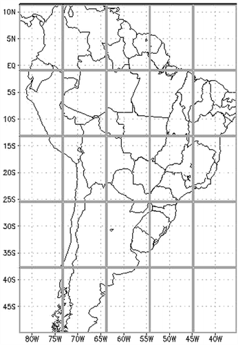
The South American region is divided into 25 sub-domains (boxes) (Figure 2). Each box has 38 points on direction x (longitude) and 49 points on direction y (latitude), representing a total of 9.5° of longitude and 12.25° of latitude (horizontal resolution with 0.25°).

4. Results

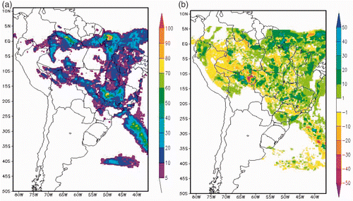
For the period of simulation, the precipitation field estimated by the TRMM satellite is shown in Figure 3(a). There is a precipitation region crossing South America from the northwest (on the Equator) to the southeast (Rio de Janeiro state, Brazil). This precipitation pattern is a characteristic from a SCAZ event, during 5 days over the region. According to Climálise 55, two SCAZ events were verified in February 2004. One of them had occurred during the period 20–24, where the precipitation maxima were over the South Atlantic ocean.

Figure 3. (a) Accumulated precipitation for 24 h (mm) on 21 February 2004 estimated by TRMM satellite, applying 3B42_RT algorithm and (b) simulated precipitation by BRAMS (mm) using ENS approach for the same day.

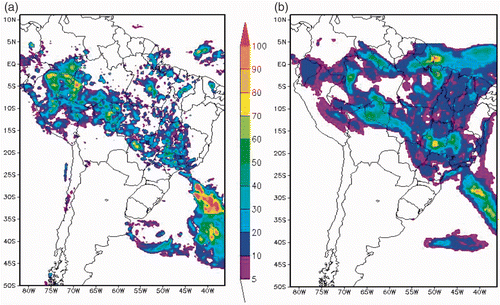
The simulation of the BRAMS model using the ENS approach (Figure 3b) shows the performance of the model to reproduce the large-scale characteristic associated to the space pattern of the precipitation distribution on the SCAZ event. However, there is an over-estimation of the precipitation on the most part of Brazil, and also over the Intertropical Convergence Zone (ITCZ). On the other hand, the model under-estimated the precipitation over the west part for the Amazonian region.

Before applying the inversion scheme to the event shown in Figure 3, the methodology will be employed to identify synthetic precipitation.

The estimated precipitation field P_S, from Equation (4) and the observed precipitation are shown in Figure 3. The FA is employed to compute the model precipitation (Figure 4b).

Figure 4. (a) Synthetic precipitation field (mm) and (b) estimated precipitation field (mm).

Looking at the estimated weights in Table 2, it could be considered a very good estimation. However, precipitation is a very sensitive variable. The ensemble approach to the convection was able to give a good qualitative distribution of the precipitation, but there is a difference between the estimated and observed precipitation fields (Figure 4).

Table 2. Estimated weights by the FA.

Parameterizations	True weight	Estimated weight
WAS	0.25	0.26
WGR	0.35	0.36
WKF	0.20	0.18
WMC	0.15	0.16
WLO	0.05	0.04

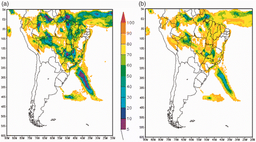
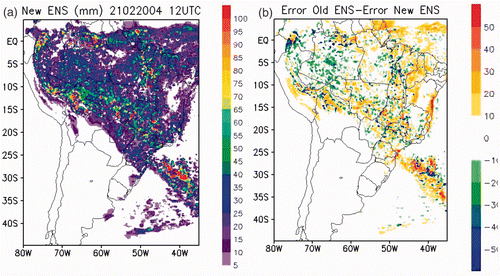
The second experiment was carried out using TRMM satellite data. The estimated precipitation field (Figure 5a) presents the same space pattern simulated by ENS, but the weighted estimation gives a finer adjustment, minimizing the over-precipitation over the central region of Brazil and on ITCZ. Figure 4(b) shows the absolute difference between the observed and estimated precipitations. The weighted ensemble estimation produced an under-estimation over the west part for the Amazon river basin.

Figure 5. (a) Total precipitation estimated by 24 h of simulation on 21 February 2004 (mm) and (b) difference for total precipitation by ENS approach and the weighted ensemble estimation.

For the new weighted ensemble approach, the over-estimation for precipitation persists, but it is reduced. Figure 6 presents the m_b for the F-ENS (Firefly ENS), showing a reduction for the over-precipitation, in comparison with standard ENS (Figure 3). From the analysis of the absolute errors for the convective precipitation fields obtained from standard ENS (Figure 2b) and the weighted parameterization, the results obtained with the methodology introduced here were improved.

Figure 6. Convective precipitation (mm) simulated by BRAMS model: (a) weighted estimation and (b) field of difference.

Table 3 presents the scores computed in each box over the evaluated domain. The indices x_i, x_e and y_i, y_e represent, respectively, the first point and end point in the x and y directions. In a total of 25 boxes, 14 were marked by high scores using the precipitation retrieved and 11 using the ensemble mean precipitation. However, when the precipitation retrieved showed low scores, the ensemble mean showed very high scores.

Table 3. BRAMS model total precipitation RMS error and Bias for: ensemble simple mean (ENS) and precipitation retrieved using the FA (FY).

xi	xe	yi	ye	Ensemble mean		Retrieved
				Bias (ENS)	RMS (ENS)	Bias (FY)	RMS (FY)
1	38	1	49	−0.145	3.302	0.655	3.606
1	38	50	98	0.136	1.798	0.003	0.032
1	38	99	147	−0.965	4.342	−0.843	4.252
1	38	148	196	−9.180	19.467	−9.386	17.878
1	38	197	245	0.288	8.403	3.530	14.349
39	76	1	49	0.131	0.678	0.623	2.313
39	76	50	98	−0.521	1.693	0.248	4.657
39	76	99	147	−0.155	3.857	0.153	5.288
39	76	148	196	−7.158	23.874	−17.014	26.038
39	76	197	245	1.767	15.720	−0.081	10.183
77	114	1	49	−0.719	3.154	3.865	10.413
77	114	50	98	−0.315	1.930	−0.320	1.918
77	114	99	147	−0.973	11.409	−4.291	13.348
77	114	148	196	4.072	13.061	−6.248	16.701
77	114	197	245	10.594	17.541	3.429	8.112
115	152	1	49	−1.756	9.675	−3.928	10.663
115	152	50	98	0.471	2.501	1.111	5.570
115	152	99	147	5.735	19.330	−3.378	20.602
115	152	148	196	7.198	16.057	0.956	18.387
115	152	197	245	25.213	31.229	1.576	11.262
153	190	1	49	−13.035	23.109	−15.302	24.967
153	190	50	98	−11.930	33.893	−29.889	46.103
153	190	99	147	5.647	9.162	10.342	18.581
153	190	148	196	8.611	12.299	0.442	7.517
153	190	197	245	15.663	20.765	−1.122	12.692

5. Final considerations

In this article, the precipitation field is computed from a multi-model ensemble approach, where the final calculation is given by a weighted average from different parameterizations for the rainfall. The numerical values of the weights for such average are addressed formulating the problem as minimizing the generalized functional of least square between the precipitation computed from five different parameterizations and satellite data. The firefly meta-heuristic is employed to solve the optimization problem. The methodology was tested using the meteorological meso-scale BRAMS over South America on the period of SCAZ event: from 20 up to 24 February, 2004.

Two numerical experiments were carried out. The first one employed synthetic observations. In the second experiment, the precipitation field was calculated using TRMM data.

The results obtained with synthetic observation data indicates that FA depends on numerical values of some parameters: the number of individuals in the firefly population and the number of iterations. Some tests were carried out to determine good values for these parameters. The weights were identified with very good precision. For improving the precision, other stopping criterion could be studied.

Considering the experiment using TRMM data, the estimated precipitation is closer to the observed field. According to the error field, the absolute error of the estimated precipitation field is less than that computed by ENS. However, the goal is not to retrieve the precipitation field, but apply the computed weights into meteorological computer code BRAMS. Therefore, a computation for the new mass flux m_b is also done. The weighted ensemble average obtained by the firefly optimization presents an impact on the precipitation fields simulated by the BRAMS. The reduction on the precipitation is not significant in those regions where the rainfall was not observed. However, this new methodology acts by minimizing the over-estimation on several regions.

The results encourage the application of numerical methodologies for solving this inverse problem of parameter estimation. The next step in this investigation is to employ a larger period of simulations for obtaining a weight set with more number of weights available for different seasons in the year.

The main goal of this article is to improve the performance of the atmospheric modelling in CPTEC–INPE. A better representation of deep convection in the numerical models is a contribution to enhance the skills of the numerical weather prediction and air quality monitoring by the BRAMS model. Future work will apply the same methodology to the Global Atmospheric Circulation Model from the CPTEC–INPE.

Acknowledgements

Ariane F. dos Santos was supported by Fundação de Amparo à Pesquisa do Estado de São Paulo (FAPESP), process 2008/01983-0. Authors Ariane F. dos Santos, Haroldo F. de Campos Velho, Saulo R. Freitas, Manoel A. Gan thank the Brazilians Federal (CNPq and CAPES) and State (FAPESP) agencies for supporting the study.

References

- C.E.M. Tucci, Modelos Hidrológicos, ABRH Editora da UFRGS, Porto Alegre, 1998 (in Portuguese).
- Vila, DA, de Gonçalves, LGG, Toll, DL, and Rozante, JR, 2009. Statistical evaluation of combined daily gauge observations and rainfall satellite estimates over continental South America, J. Hydrometeorol. 10 (2009), pp. 533–543.
- A. Arakawa, Modelling clouds and cloud processes for use in climate model. The Physical Basis of Climate and Modelling, GARP Publication Series, no. 16, WMO, Geneva, 1975, pp. 183–197.
- W.R. Cotton and R.A. Anthes, Storm and Cloud Dynamics, Academic Press, San Diego, CA, 1989. (International Geophysics Series, Vol. 44).
- K. Ooyama, A theory on parameterization of cumulus convection, J. Meteorol. Soc. Jpn. 39 (Special issue) (1971), pp. 744–756.
- Arakawa, A, and Schubert, EWH, 1974. Interaction of a cumulus cloud ensemble with the large-scale environment, Part I, J. Atmos. Sci. 31 (1974), pp. 674–701.
- Kuo, HL, 1974. Further studies of the parameterization of the influence of cumulus convection on large-scale flow, J. Atmos. Sci. 31 (1974), pp. 1232–1240.
- Betts, AK, 1986. A new convective adjustment scheme. Part I: Observational and theoretical basis, Q. J. R. Meteorolog. Soc. 112 (1986), pp. 677–691.
- Grell, G, 1993. Prognostic evaluation of assumptions used by cumulus parameterizations, Mon. Weather Rev. 121 (1993), pp. 764–787.
- Grell, GA, and Dévényi, D, 2002. A generalized approach to parameterizing convection combining ensemble and data assimilation techniques, Geophys. Res. Lett. 29 (14) (2002), pp. 1693–1694.
- Freitas, SR, Longo, KM, Silva Dias, MAF, Chatfield, R, Silva Dias, P, Artaxo, P, Andreae, MO, Grell, G, Rodrigues, LF, Fazenda, A, and Panetta, J, 2009. The coupled aerosol and tracer transport model to the Brazilian developments on the regional atmospheric modeling system (CATT-BRAMS) – Part 1: Model description and evaluation, Atmos. Chem. Phys. 9 (2009), pp. 2843–2861.
- Kain, JS, and Fritsch, JM, 1992. The role of the convective trigger function in numerical forecasts of mesoscale convective systems, Meteorol. Atmos. Phys. 49 (1992), pp. 93–106.
- Brown, JM, 1979. Mesoscale unsaturated downdrafts driven by rainfall evaporation: A numerical study, J. Atmos. Sci. 36 (1979), pp. 313–338.
- Krishnamurti, TN, Low-nam, S, and Pasch, R, 1983. Cumulus parameterizations and rainfall rates II, Mon. Weather Rev. 111 (1983), pp. 815–828.
- Freitas, SR, Longo, K, Dias, MS, Dias, PS, Chatfield, R, Prins, E, Artaxo, P, Grell, G, and Recuero, F, 2005. Monitoring the transport of biomass burning emissions in South America, Environ. Fluid Mech. 5 (2005), pp. 135–167.
- Gevaerd, R, Freitas, SR, Longo, M, Moreira, DS, Silva Dias, MA, and Silva Dias, P, 2006. Estimativa operacional da umidade do solo para iniciação de modelos de previsão numérica da atmosfera. Parte II: Impacto da umidade do solo e da parametrização de cumulus na simulação de uma linha seca, Rev. Bras. Meteorol. 21 (3a) (2006), pp. 74–88.
- Beck, JV, Blackwell, B, and Clair, C.R., 1985. Inverse Heat Conduction: Ill-Posed Problems. New York: John Wiley & Sons; 1985.
- Twomey, S, 1977. Introduction to the Mathematics of Inversion in Remote Sensing and Indirect Measurements. Amsterdam: Elsevier Scientific; 1977.
- Liou, KN, 1982. An Introduction to Atmospheric Radiation. Orlando, FL: Academic Press; 1982.
- J.C. Carvalho, Inferência de perfis verticais de temperatura utilizando uma técnica iterativa implícita de inversão, M.Sc. thesis (Meteorology), INPE, São José dos Campos (Brazil), 1998 (in Portuguese).
- J.C. Carvalho, Modelagem e análise de sondagens remotas sobre o Brasil utilizando-se o sistema ICI, D.Sc. thesis (Meteorology), INPE, São José dos Campos (Brazil), 2002 (in Portuguese).
- Ramos, FM, Campos Velho, HF, Carvalho, JC, and Ferreira, NJ, 1999. Novel approaches on entropic regularization, Inverse Probl. 15 (1999), pp. 1139–1148.
- E.H. Shiguemori, Recuperação de perfis de temperatura e umidade da atmosfera a partir de dados de satélite – abordagens por redes neurais artificiais e implementação em hardware, D.Sc. thesis (Applied Computing), INPE, São José dos Campos (Brazil), 2007 (in Portuguese).
- Shiguemori, EH, Da Silva, JDS, Campos Velho, HF, and Carvalho, JC, 2008. Atmospheric temperature retrieval by a radial basis function neural network, Int. J. Inf. Commun. Technol. 1 (2008), pp. 224–239.
- H.H. Barboza, C. De, A.L. Bortoli, R.D. Cunha, and J.C. Simoes, Simulação bidimensional do fluxo da geleira Lange, ilha Rei George, Antártica, TEMA 4(2) (2003), pp. 159–166 (in Portuguese).
- Daley, R, 1991. Atmospheric Data Analysis. Cambridge: Cambridge University Press; 1991.
- Kalnay, E, 2003. Atmospheric Modeling, Data Assimilation and Predictability. Cambridge: Cambridge University Press; 2003.
- Zannetti, P, 1990. Air Pollution Modeling. Theories, Computational Methods and Available Software. New York: Kluwer Academic; 1990.
- P. Kashibathla, M. Heimann, P. Rayner, N. Mahowald, R.G. Prinn, and D.E. Hartley (eds.), Inverse Methods in Global Biogeochemical Cycles, Geophysical Monograph 114, American Geophysical Union, Washington, DC, 2000.
- D.R. Roberti, Problemas inversos em física da atmosfera. Santa Maria, D.Sc. thesis (Physics), Centro de Ciências Naturais e Exatas, Universidade Federal de Santa Maria (Brazil), 2005 (in Portuguese).
- Roberti, DR, Anfossi, D, Campos Velho, HF, and Degrazia, GA, 2007. Estimation of pollutant source emission rate from experimental data, Nuovo Cimento Soc. Ital. Fis. C 30 (2007), pp. 177–186.
- Bocquet, M, 2005. Reconstruction of an atmospheric tracer source using the principle of maximum entropy, I: Theory, Q. J. R. Meteorolog. Soc. 131 (2005), pp. 2191–2208.
- E.F.P. Luz, H.F. de Campos Velho, J.C. Becceneri, and D.R. Roberti, Estimating atmospheric area source strength through particle swarm optimization. In: Inverse Problems, Desing and Optimization Symposium, Miami (IPDO-2007), Vol. 1, 2007, pp. 354–359.
- Tikhonov, AN, and Arsenin, VY, 1977. Solution of Ill-Posed Problems. New York: Winston and Sons; 1977.
- H.F. de Campos Velho, Problemas Inversos em Pesquisa Espacial, Sociedade Brasileira de Matematica Aplicada e Computacional, Sao Carlos, 2008.
- H.F. Campos Velho, Inverse problems in space research, Brazilian Society for Computational and Applied Mathematics (SBMAC), São Carlos, 2008 (in Portuguese).
- Yang, X, 2008. Nature-Inspired Metaheuristic Algorithms. London: Luniver Press; 2008.
- Gevaerd, R, and Freitas, SR, 2006. Estimativa operacional da umidade do solo para iniciação de modelos de previsão numérica da atmosfera. Parte I: Descrição da metodologia e validação, Rev. Bras. Meteorol. 21 (3a) (2006), pp. 59–73.
- Mellor, GL, and Yamada, T, 1982. Development of a turbulence closure model for geophysical fluid problems, Rev. Geophys Phys. Space Phys. 20 (1982), pp. 851–875.
- J.S. Olson, Global ecosystem framework-definitions, USGS EROS Data Center Internal Report, Sioux Falls, SD, 1994.
- Proveg. Atualização da Representação da vegetação nos Modelos Numéricos do CPTEC, 2005, Available at www.cptec.inpe.br/proveg.
- M.F. Sestini, É.S. Reimer, D.M. Valeriano, R.C.S. Alvalá, E.M.K. Mello, C.S. Chan, and C.A. Nobre, Mapa de cobertura da terra da Amazônia Legal para uso em modelos meteorólogicos, in Simpósio Brasileiro de Sensoriamento Remoto 11 (SBSR), 2003, Belo Horizonte, Anais, INPE, São José dos Campos, 2003. pp. 2901–2906. Available http://urlib.net/rep/ltid.inpe.br/sbsr/2002/11.22.20.34?languagebutton=pt-BR“\n_blankhttp://urlib.net/ltid.inpe.br/sbsr/2002/11.22.20.34..
- Walko, R, Band, L, Baron, J, Kittel, F, Lammers, R, Lee, T, Ojima, D, Pielke, R, Taylor, C, Tague, C, Tremback, C, and Vidale, P, 2000. Coupled atmosphere-biophysics-hydrology models for environmental modeling, J. Appl. Meteorol. 39 (2000), pp. 931–944.
- R.L. Walko and C.J. Tremback, Modifications for the transition from LEAF-2 to LEAF-3, ATMET Technical Note, ATMET, Boulder, CO.
- Walko, RL, Cotton, WR, Meyers, MP, and Harrington, JY, 1995. New RAMS cloud microphysics parameterization. Part I: the single-moment scheme, Atmos. Res. 38 (1995), pp. 29–42.
- Meyers, MP, Walko, RL, Harrington, JY, and Cotton, WR, 1997. New RAMS cloud microphysics parameterization. Part II: The two-moment scheme, Atmos. Res. 45 (1997), pp. 3–39.
- S. Freitas, G. Grell, R. Gevaerd, and K. Longo. Simulating typical rainfall systems on South America using an ensemble version of convective parameterization, 3rd Pan-GCSS meeting on “Clouds, Climate and Models”, Athens, Greece, 2005.
- A.C. Vasques, Características de precipitação sobre a América do Sul proveniente de diferentes fontes de dados com ênfase no Brasil, M.Sc. thesis (Meteorology), INPE, São José dos Campos, 2007 (in Portuguese).
- C.M. Santos e Silva, Simulando o ciclo diário da precipitação sobre a Bacia Amazonica durante a estação chuvosa, D.Sc. thesis (Meteorology), INPE, São José dos Campos (Brazil), 2009 (in Portuguese).
- S. Arya, D.M. Mount, N.S. Netanyahu, R. Silverman, and A.Y. Wu, An optimal algorithm for approximate nearest neighbor searching in fixed dimensions, J. ACM 45(6) (1998), pp. 891–923. Available at http://www.cs.umd.edu/~mount/Papers/dist.pdf.
- Yang, X-S., 2010. Firefly algorithm, stochastic test functions and design optimisation, Int. J. of Bio-Insp. Comp. 2 (2010), pp. 78–84.
- E.F.P. Luz, J.C. Becceneri, and H.F.C Velho, Recuperação da Condição Inicial da Equação do Calor com o Uso da Metaheurística Firefly Algorithm. In: Congresso Nacionalde Matemática Aplicada e Computacional, 33 (CNMC), 2010, Águas de Lindóia, 20–23 September 2010. DVD.
- A.F. Santos, S.R, Freitas, E.F.P. Luz, H.F. De Campos Velho, and M.A. Gan, Optimization firefly method for weighted ensemble of convective parameterizations. Part II: Sensitivity experiment using TRMM satellite data, AGU-2010 Meeting of the Americas, Foz do Iguaçu, 2010.
- A.F. Santos, S.R. Freitas, E.F.P. Luz, H.F. De Campos Velho, and M.A. Gan, Optimization firefly method for weighted ensemble of convective parameterizations. Part I: Results with a synthetic precipitation field, AGU-2010 Meeting of the Americas, Foz do Iguaçu, 2010.
- Climanálise, Boletim de Monitoramente e Análise Climática, 20(2), February 2004.