An a posteriori truncation method for some Cauchy problems associated with Helmholtz-type equations

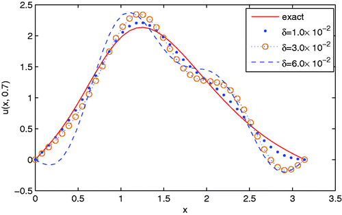
Abstract

In this article, we investigate some Cauchy problems associated with Helmholtz-type equations in rectangle using the method of truncation. Not alike the previous literature, we propose to choose the regularization parameter by an a posteriori rule, with which we can obtain error estimates of Hölder-type between the exact solution and their regularized approximation. Numerical simulations show that the proposed scheme is effective and stable.

Keywords:

• ill-posed problems
• regularization
• Cauchy problem
• a posteriori choice
• Helmholtz-type equation

1. Introduction

The Helmholtz-type equation in an open bounded domain Ω ⊂ ℝ² can be formulated as 1(1) where Δ is the two-dimensional Laplace operator, and is known as wave number. For the case α ∈ ℝ, β = 0, Equation (1.1) is usually known as the Helmholtz equation; it is frequently encountered in many scientific and engineering areas, for example it can be used to describe vibration of a structure 2, the acoustics cavity problem 3, wave propagation and scattering 4–6. For the case α = 0, β ∈ ℝ, Equation (1.1) is the so-called modified Helmholtz equation or Yukawa equation 7; it appears, for instance, in the semi-implicit temporal discretization of the heat or the Navier–Stokes equations 8 and it can also be used to model the heat conduction in a fin 9. Meanwhile, the well-studied Laplace equation is a special case of Equation (1.1) with α = 0, β = 0.

The direct problems of the Helmholtz-type equation, i.e. Equation (1.1) with Dirichlet, Neumann or mixed boundary conditions specified on the whole boundary ∂Ω, have been investigated extensively in the past years. However, in some practical applications, the boundary data on the entire boundary cannot be acquired due to technical difficulties. We only know the noisy data on a part of the boundary of the concerning domain, which leads to some inverse problems, including the Cauchy problem as a particular case.

The Cauchy problems for the Helmholtz equation 10, the modified Helmholtz equation and the Laplace equation are well known to be severely ill-posed in the sense of Hadamard, i.e. small disturbance in the data may be dramatically magnified in the solution. Until the present moment, there has been a huge number of literature on them, here we shall only give a partial list of the references: see, for example 11–20 for the Helmholtz equation, 1,21–26 for the modified Helmholtz equation and 27–36 for the Laplace equation. However, due to the authors' knowledge, there are much fewer papers devoted to error estimates using regularization methods with a posteriori parameter choice rule, under which the a priori information, such as the smoothness of the unknown exact solution, is no needed for computing the regularization parameter. This is very important, because the a priori information of the solution is unknown for most practical engineering and scientific problems.

In this article, we firstly consider the Cauchy problem for the Helmholtz equation in a rectangle using the truncation method (TM) with an a posteriori parameter choice rule, with which we obtain the error estimate of Hölder-type between the exact solution and the regularized solution. Then the similar error estimates for the Cauchy problems for the modified Helmholtz equation and the Laplace equation can be obtained as direct corollaries of the foregoing result. It should be pointed out that a similar approach to choose the regularization parameter has been successfully applied to numerical differentiation and numerical analytic continuation in the recent papers 37,38 based on Hermite functions expansion.

The rest of this article is organized as follows. In Section 2, we give the mathematical formulation of the considered problems and some preliminaries. The regularization parameter choice rule and the error estimates are presented in Section 3. In Section 4, some simple numerical examples are given to test the accuracy, stability and efficiency of the proposed method. Section 5 ends this article with a short conclusion.

2. Mathematical problem and preliminaries

Let L²(0, π) be a Hilbert space, for any function w(x) ∈ L²(0, π), , is the inner product in L²(0, π). For simplicity, we will, respectively, write ‖ · ‖ and ⟨·, ·⟩ for and hereinafter.

We consider the following Cauchy problem for the Helmholtz equation at first:(2) where constant k = α + βi with β = 0 is the wave number. Here, we only consider the case of α ∈ ℝ⁺.

Assume that the exact data ϕ ∈ L²(0, π) and the measured data ϕ^δ ∈ L²(0, π), which satisfy(3) where δ > 0 is the noise level. For the purpose of theory analysis, we further assume that u(·, y) ∈ L²(0, π) for 0 ≤ y ≤ 1 and there exists a constant E > 0 such that the following a priori bound holds,(4)

By the method of separation of variables, the solution of problem (2.1) can be obtained as follows 16,(5) where , ϕ_n = ⟨ϕ, X_n⟩ and (n = 1, 2, …) form a standard orthogonal system of L²(0, π). In practical problems, α is a fixed constant, and the formula ⌊α⌋ denotes the largest integer smaller than or equal to α.

Due to (2.4) and Parseval formula, we have(6) The formula (2.3) implies that the Fourier coefficients ϕ_n must decay rapidly for large n, since the factor as n → ∞ for α ∈ ℝ⁺. However, in practice, the data is inevitably contaminated by noise, and then such a decay of exact data can not be expected for the Fourier coefficients of the measured data ϕ^δ(x). Thus, a small perturbation of the data ϕ(x) may be severely magnified in the solution u(x, y) for 0 < y < 1. This is just the essential reason of the ill-posedness of Cauchy problem for the Helmholtz equation. A natural way to recover the stability of problem (2.1) is to cut-off the Fourier coefficients of the noisy data appropriately. Under the scenario of a priori parameter choice, this idea has been successfully applied to solve Cauchy problems for the Helmholtz equation 16, the modified Helmholtz equation 23 and the Laplace equation 35. Yet, there is not any result using TM with a posteriori parameter choice rule, we will give an a posteriori rule on how to choose the regularization parameter N and give the corresponding error estimates in the next section.

3. An a posterior parameter choice and the error estimates

Let N be a positive integer and P_N: L²(0, π) → span{X_n(x)|n ≤ N} is an orthogonal projection. Then, based on the analysis in Section 2, for proper large α, we define the regularized solution of problem (2.1) corresponding to the noisy data as , i.e.(7) where N is the regularization parameter.

Similar to 37,38, for a given δ, we propose to choose the number of the Fourier coefficients as the first integer N such that ‖(I − P_N)ϕ^δ‖ ≤ τδ (τ > 1), i.e.(8) Note that the integer N satisfies (3.2) will be dependent on the given tolerance δ, to emphasis this dependent relationship, we denote it N(δ) in the following.

Remark 3.1

The parameter τ > 1 should be a fixed constant with proper quantity. On the one hand, if τ ≤ 1, then for a given small tolerance δ, the integer N(δ) chosen according to (3.2) might be too large, which makes the approximation loose the regularization effect. On the other hand, if τ is too large, then the integer N(δ) chosen according to (3.2) might be quite small, which means that the approximation inherits too less information from the data, and leads to an unacceptable deviation between the approximation and the objective solution.

Proposition 3.2

Let u(x, y) be the solution of problem (2.1) and the conditions (2.2), (2.3) be satisfied. If the regularization parameter N(δ) is chosen according to (3.2), then there holds(9)

Proof

From (2.2) and (3.2), we have

Meanwhile, for 0 < α < 1,i.e.

For 1 ≤ α ≤ N(δ), we can get the same estimate. Thus, we havei.e.The proof is completed.▪

Proposition 3.3

Let all the conditions in Proposition 3.2 be satisfied. If u_N(δ)(x, y) = P_N(δ)u(x, y), then there holds the following estimate(10)

Proof

For 0 < α < 1, ∀y ∈ (0, 1), using Parseval formula and Hölder inequality, we haveBy (3.2), it follows thati.e.For the case of 1 ≤ α ≤ N(δ), the same estimate can also be derived.▪

Proposition 3.4

Let u(x, y) be the solution of (2.1), and the conditions (2.2), (2.3) be satisfied. If the regularized solution of problem (2.1) is defined by (3.1) with N(δ) chosen according to (3.2), then there holds the following estimate(11)

Proof

For the case of 0 < α < 1,

For the case of 1 ≤ α ≤ N(δ),

Combining the above two cases, the proof of this proposition is completed.▪

Theorem 3.5

Let all the conditions in Propositions 3.2–3.4 be satisfied. If the regularization parameter N(δ) is chosen according to (3.2), then for α ≤ N(δ) and ∀y ∈ (0, 1), there holds the following error estimate between the exact solution and its regularized approximation:(12)

Proof

Combine Propositions 3.2–3.4, the result (3.6) is obvious.▪

Remark 3.6

It should be noted that we cannot get the convergence analysis for y = 1. For this case, much stronger a priori information must be assumed, for example . However, we do not pursue this here.

Corollary 3.7

When k = 0, problem (2.1) is the Cauchy problem for the Laplace's equation. For this special case, the exact solution (2.4) becomes . We define the regularization solution asIf the regularization parameter N(δ) is chosen according to (3.2), then there holds the following estimate of Hölder type(13) where .

Corollary 3.8

When the wave number k = α + βi with α = 0 and β ∈ ℛ⁺, problem (2.1) is the Cauchy problem for the modified Helmholtz equation. The exact solution for this problem is . If we defineas the approximate solution, and choose the regularization parameter N(δ) according to (3.2), then there also holds the following estimate of Hölder type(14) where C is the same as in Corollary 3.7.

Remark 3.9

The proof processes of Corollaries 3.7 and 3.8 are the same as Propositions 3.2–3.4, we omit them here.

Remark 3.10

The general case of the Cauchy problems for the Helmholtz-type equations (k = α + iβ, α, β ∈ ℝ) with non-homogeneous Dirichlet data and non-homogeneous Neumann data can be expressed as follows:(15) Based on the above discussions and the principle of superposition, it is enough to consider the following Cauchy problem with homogeneous Dirichlet data and non-homogeneous Neumann data:(16) Under the a priori scenario, problem (3.10) with α ∈ ℝ⁺ and β = 0 has been considered in 39, but it was solved by quasi-reversibility method. We are pretty sure that our techniques in this article can also be parallelly applied to problem (3.10). Instead of giving the specific theoretic estimates, we present a numerical example using the a posteriori truncation method in Section 4 as a validation.

4. Numerical simulations

In this section, we will give some simple examples to illustrate the accuracy and efficiency of the truncation regularization method with a posteriori rule (3.2). For all of the following examples, the simulated data are generated using the following formula:(17) where φ is the exact data and randn(size(φ)) is white noise, the magnitude δ indicates the noise level of the measured data.

For fixed y ∈ (0, 1), in order to measure the accuracy of the numerical approximation of the function u(x, y), we use the relative root mean square error (RRMSE) defined as(18) where u and are the exact solution and the approximation, respectively. In all of the examples considered hereinafter, M is taken to be 41.

For evaluation of all the Fourier coefficients involved in the examples, we use the Simpson formula to calculate the integrals ϕ_n = < ϕ, X_n > (n = 1, 2, … , N₀) in [0, π], and the coefficients corresponding to the noisy data ϕ^δ are also computed in the same way, where N₀ is a sufficiently large positive integer.

To compute the regularization parameter, we always choose N(δ) according to (3.2), where the constant τ > 1 can be taken heuristically to be 1.01, as suggested by Hanke and Hansen 40.

In the following, we will give four numerical examples to show the stability and robustness of the method proposed in this article. Both Examples 4.1 and 4.2 are illustrations for the Cauchy problem for the Helmholtz equation, where Example 4.1 is with non-homogeneous Dirichlet data and homogeneous Neumann data, and Example 4.2 is with homogeneous Dirichlet data and non-homogeneous data. Examples 4.3 and 4.4 are illustrations for the Cauchy problems for the modified Helmholtz equation and the Laplace equation, respectively.

Example 4.1

We consider the following direct problem at first:(19) where α ∈ ℝ⁺. Similar to 16, by the method of separation of variables, the solution of problem (4.3) is as follows,(20) where and .

Hence, by (4.4), we have(21) Note that the above formula on u(x, 0) is an infinite series, for the purpose of the practical computation, we need to cut off it as(22) for sufficiently large N₀. In our computation, we take N₀ = 20 and keep this number for all the following examples. Let ϕ₁(x) ≔ ũ(x, 0), and be computed according to (4.1).

For every y ∈ (0, 1), the exact solution u(x, y) and the regularization approximation for the following Cauchy problem for the Helmholtz equationare computed by(23) and(24) respectively.

Figure 1(a) is the absolute error between the exact solution and the approximation obtained by (3.1) with N = N₀ for Example 4.1, where the noise level is δ = 1.0 × 10⁻² and α = 2.5. From this figure, we know that the absolute error even up to 10⁴ for y near to 1. Figure 1(b) shows the relationship between the RRMSE and different values of N, here y = 0.9, α = 2.5 and δ = 1.0 × 10⁻². These two figures show that an appropriate cut-off of the number of the Fourier coefficients is necessary, and this is just the main aim of this article.

Figure 2(a) is the contours of the exact solution (solid line) and the regularization solution (dash line) for Example 4.1, Figure 2(b) is the error , the noise level is δ = 1.0 × 10⁻². From these figures, it can be seen that, on the whole, the regularization solution approximates the exact solution well, particularly, these two figures show that the regularization parameter plays a key role in the process of computation.

Under the scenario of a priori parameter choice, 16 proposed to choose the regularization parameter as for p = 0. Figure 2(c) gives the comparison between the exact solution and the approximations with a priori and a posteriori parameter choice rule, here we compute E using the command norm(·, 2) in matlab 7.04, and α = 2.5, δ = 1.0 × 10⁻². Figure 2(d) shows the comparisons between the exact solution and corresponding approximation for different values of y with α = 0.5, δ = 5.0 × 10⁻².

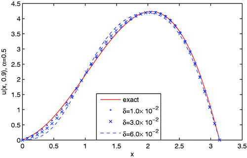
Figure 3 presents the comparisons between the exact solution and the regularization solution with different amount of noise levels added into the data, here the wave number α is also taken to be 0.5, y = 0.9. It is easy to see from this figure that the regularization solution approximates the exact solution well even for noise level up to 6.0 × 10⁻².

Figure 1. (a) The absolute error between the exact solution u(x, y) and the solution u^δ(x, y) without regularization for Example 4.1, the noise level is δ = 1.0 × 10⁻² and α = 2.5. (b) RRMSE with respect to different values of N, where α = 2.5, y = 0.9, δ = 1.0 × 10⁻².

Figure 2. (a) The contours of the exact solution (solid) and the regularization solution (dash) for Example 4.1, the noise level is δ = 1.0 × 10⁻² and α = 2.5. (b) The error for Example 4.1, the noise level is δ = 1.0 × 10⁻² and α = 2.5. (c) The comparison between the exact solution and the approximations with a priori rule and a posteriori rule, the noise level is δ = 1 × 10⁻² and y = 0.9, α = 2.5. (d) The comparisons between the exact solution and the regularization solution with respect to different values of y for Example 4.1, the noise level is δ = 5.0 × 10⁻² and α = 0.5.

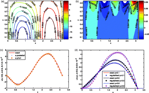
Figure 3. The comparisons between the exact solution and the regularization solutions with respect to different amount of noise levels added into the Cauchy data for Example 4.1, where y = 0.9 and α = 0.5.

Example 4.2

Consider the following Cauchy problem for the Helmholtz equation with non-homogeneous Neumann data:(25)

Here, we take α = 0.5, for example, similar to the construction process in Example 4.1. If we take u_y(x, 1) = x²(π − x) and chooseand let be generated according to (4.1), then the exact solution and regularized solution of (4.9) can be, respectively, computed asand

The numerical results for Example 4.2 are illustrated in Figure 4. Figure 4(a) shows the comparison between the exact solution (solid) and the regularization solution (dash), the noise level is δ = 1.0 × 10⁻². Figure 4(b) presents the algebraic error , the noise level is δ = 1.0 × 10⁻². Figure 4(c) is the comparison between the exact solution and the regularization solution with respect to different values of y, here the noise level is 5.0 × 10⁻². Figure 4(d) shows the comparisons between the exact solution and the regularization solution with noise level δ ∈ {1.0 × 10⁻², 3.0 × 10⁻², 6.0 × 10⁻²}, y = 0.9. From these figures, it can be seen that the a posteriori truncation method proposed in this article works very well for the Cauchy problem for the Helmholtz equation with non-homogeneous Neumann data, which verifies our assertion in Remark 3.10. For simplicity we only provide the Cauchy problems for the modified Helmholtz equation and the Laplace equation with homogeneous Neaumann data in the following.

Figure 4. (a) The contour of the exact solution (solid) and the regularization solution (dash) for Example 4.2, the noise level is δ = 1.0 × 10⁻². (b) The error for Example 4.2, the noise level is δ = 1.0 × 10⁻². (c) The comparison between the exact solution and the regularization solution with respect to different values of y for Example 4.2. (d) The comparison between the exact solution and the regularization solution with respect to different amount of noise levels added into the Cauchy data for Example 4.2.

Example 4.3

Consider the following Cauchy problem for the modified Helmholtz equation with β = 2,(26) If we choose u(x, 1) = x²(π − x)² and letAssume is also generated according to (4.1), then the exact solution and the regularized solution for (4.10) can be computed asand

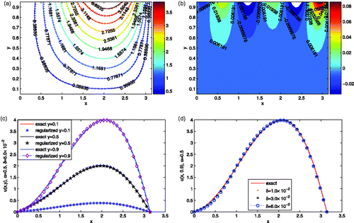
In 23, for p = 0, the authors suggested to choose the regularization parameter by a priori rule as(27) The comparison of the regularization solutions with the a posteriori choice rule (3.2) and the a priori choice rule (4.11) is shown in Figure 5(c).

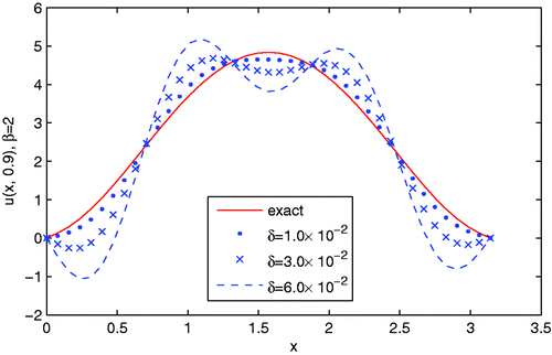
Other numerical simulations for this example are showed in Figures 5(a), (b), (d) and 6. Particularly, from Figures 5(d) and 6, it can be seen that the numerical effect gets worse with respect to increasing the value of y and the value of noise level.

Figure 5. (a) The contours of the exact solution (solid) and the regularization solution (dash) for Example 4.3, the noise level is δ = 1.0 × 10⁻². (b) The error for Example 4.3, the noise level is δ = 1.0 × 10⁻². (c) The comparisons between the exact solution and approximation with a priori rule and a posteriori rule for Example 4.3, the noise level is δ = 1.0 × 10⁻² and y = 0.9. (d) The comparisons between the exact solution and the regularization solution with respect to different values of y for Example 4.3, the noise level is δ = 5.0 × 10⁻². The value of β for all the four figures is chosen to be 2.

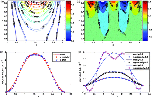
Figure 6. The comparisons between the exact solution and the regularization solution with respect to different amount of noise levels added into the Cauchy data for Example 4.3, where y = 0.9 and β = 2.

Example 4.4

In this example, we consider the following Cauchy problem for the Laplace equation(28) If we take , then by the same construction process as before, we choose , and let be computed according to (4.1). The exact solution u(x, y) and the regularization solution for problem (4.11) are computed byandrespectively.

Qian et al. 35 proposed to choose the regularization parameter as(29) for Cauchy problem for the Laplace equation in a rectangle, but they did not provide any numerical implementation there.

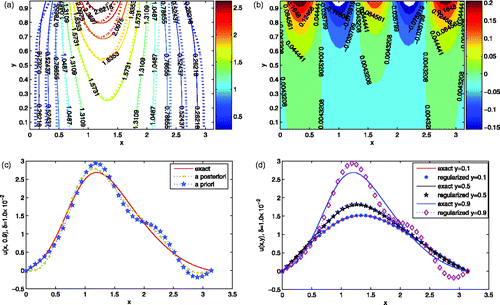
The relevant numerical results as for Example 4.3 are shown in Figures 7(a)–(d) and 8.

From the above four examples, we get the following conclusions.

1.	The proposed method in this article works well for Cauchy problems for the Helmholtz equation, the modified Helmholtz equation and the Laplace equation. The numerical results are acceptable even for the noise level added into the Cauchy data over 5.0 × 10−2.
2.	The regularization solutions obtained by a posteriori parameter choice rule are relatively better than that obtained by a priori parameter choice rule.
3.	The larger the value of y is, the worse the computational effect we can get. On the contrary, when the value of y is relatively small, especially for y = 0.1, the regularization solution is nearly coincide with the exact solution.
4.	The smaller the noise level is, the better the computational effect we can obtain.

Figure 7. (a) The contours of the exact solution (solid) and the regularization solution (dash) for Example 4.4, the noise level is δ = 1.0 × 10⁻². (b) The error for Example 4.4, the noise level is δ = 1.0 × 10⁻². (c) The comparisons between the exact solution and approximation with a priori rule and a posteriori rule for Example 4.4, the noise level is δ = 1.0 × 10⁻² and y = 0.9. (d) The comparisons between the exact solution and the regularization solution with respect to different values of y for Example 4.4, the noise level is δ = 1.0 × 10⁻².

Figure 8. The comparisons between the exact solution and the regularization solution with respect to different amount of noise levels added into the Cauchy data for Example 4.4, y = 0.7.

5. Conclusion

In this article, some Cauchy problems associated with the Helmholtz-type equations are investigated by the method of truncation. We propose to choose the regularization parameter by an a posteriori rule using the discrepancy between the noisy data and its finite dimensional projection. The corresponding error estimates between the exact solution and the regularization solution are obtained. Numerical tests show that the proposed scheme is accurate, stable and convergent with respect to decreasing the amount of noise added into the data.

Acknowledgements

The authors are indebted to the referees of this article for their most helpful comments and suggestions, which helped to improve the presentation greatly. The authors are also grateful to Dr Fan Yang for the helpful discussion during the process of amending this article.

The project is supported by the NNSF of China (No. 11171136).

References

- Marin, L, and Lesnic, D, 2005. The method of fundamental solutions for the Cauchy problem associated with two-dimensional Helmholtz-type equations, Comput. Struct. 83 (2005), pp. 267–278.
- Beskos, DE, 1997. Boundary element methods in dynamic analysis, part II (1986–1996), Appl. Mech. Rev. 50 (1997), pp. 149–197.
- Chen, JT, and Wong, FC, 1998. Dual formulation of multiple reciprocity method for the acoustic mode of a cavity with a thin partition, J. Sound Vib. 217 (1998), pp. 75–95.
- Gladwell, GML, and Willms, NB, 1995. On the mode shapes of the Helmholtz equation, J. Sound Vib. 188 (1995), pp. 419–433.
- Harari, I, Barbone, PE, Slavutin, M, and Shalom, R, 1998. Boundary infinite elements for the Helmholtz equation in exterior domains, Int. J. Num. Meth. Eng. 41 (1998), pp. 1105–1131.
- Hall, WS, and Mao, XQ, 1995. A boundary element investigation of irregular frequencies in electromagnetic scattering, Eng. Anal. Boundary Elem. 16 (1995), pp. 245–252.
- Chang, HW, Huang, JF, and Leiterman, TJ, 2006. An adaptive fast solver for the modified Helmholtz equation in two dimensions, J. Comput. Phys. 211 (2006), pp. 616–637.
- Greengard, L, and Kropinski, MC, 1998. An integral equation approach to the incompressible Navier–Stokes equations in two dimensions, SIAM J. Sci. Comput. 20 (1998), pp. 318–336.
- Kern, DQ, and Kraus, AD, 1972. Extended Surface Heat Transfer. New York: McGraw-Hill; 1972.
- Isakov, V, 1998. Inverse Problems for Partial Differential Equation. New York: Springer; 1998.
- Fu, CL, Feng, XL, and Qian, Z, 2009. The Fourier regularization for solving the Cauchy problem for the Helmholtz equation, Appl. Num. Math. 59 (2009), pp. 2625–2640.
- Hrycak, T, and Isakov, V, 2004. Increased stability in the continuation of solutions to the Helmholtz equation, Inverse Prob. 20 (2004), pp. 697–712.
- Jin, BT, and Zheng, Y, 2006. A meshless method for some inverse problems associated with the Helmholtz equation, Comput. Methods Appl. Mech. Eng. 195 (2006), pp. 2270–2280.
- Johansson, BT, and Kozlov, VA, 2009. An alternating method for Cauchy problems for Helmholtz-type operators in non-homogeneous medium, IMA J. Appl. Math. 74 (1) (2009), pp. 62–73.
- Marin, L, Elliott, L, Heggs, PJ, Ingham, DB, Lesnic, D, and Wen, X, 2003. An alternating iterative algorithm for the Cauchy problem associated to the Helmholtz equation, Comput. Methods Appl. Mech. Eng. 192 (2003), pp. 709–722.
- Qin, HH, and Wei, T, 2010. Two regularization methods for the Cauchy problems of the Helmholtz equation, Appl. Math. Model. 34 (2010), pp. 947–967.
- Regińska, T, and Regiński, K, 2006. Approximate solution of a Cauchy problem for the Helmholtz equation, Inverse Prob. 22 (2006), pp. 975–989.
- Regińska, T, and Tautenhahn, U, 2009. Conditional stability estimates and regularization with applications to Cauchy problems for the Helmholtz equation, Num. Funct. Anal. Optim. 30 (2009), pp. 1065–1097.
- Wei, T, Qin, HH, and Shi, R, 2008. Numerical solution of an inverse 2D Cauchy problem connected with the Helmholtz equation, Inverse Prob. 24 (2008), pp. 1–18.
- Xiong, XT, and Fu, CL, 2007. Two approximate methods of a Cauchy problem for the Helmholtz equation, Comput. Appl. Math. 26 (2007), pp. 285–307.
- Johansson, BT, and Marin, L, 2010. Relaxation of alternating iterative algorithms for the Cauchy problem associated with the modified Helmholtz equation, CMC: Comput. Mater. Contin. 13 (2010), pp. 153–188.
- Marin, L, 2010. An alternating iterative MFS algorithm for the Cauchy problem for the modified Helmholtz equation, Comput. Mech. 45 (2010), pp. 665–677.
- Qin, HH, and Wei, T, 2009. Quasi-reversibility and truncation methods to solve a Cauchy problem of the modifed Helmholtz equation, Math. Comput. Simulat. 80 (2009), pp. 352–366.
- Xiong, XT, Shi, WX, and Fan, XY, 2011. Two numerical methods for a Cauchy problem for modified Helmholtz equation, Appl. Math. Model. 35 (2011), pp. 4951–4964.
- Qian, A, Mao, JF, and Liu, LH, , A spectral regularization method for a Cauchy problem of the modified Helmholtz equation, Boundary Value Prob. (2010), 2010: 212056, doi:10.1155/2010/212056.
- Qian, A, and Wu, YJ, 2011. Optimal error bound and approximation methods for a Cauchy problem of the modified Helmholtz equation, IJWMIP 2 (2011), pp. 305–315.
- Berntsson, F, and Eldén, L, 2001. Numerical solution of a Cauchy problem for the Laplace equation, Inverse Prob. 17 (4) (2001), pp. 839–853.
- Bourgeois, L, 2006. Convergence rates for the quasi-reversibility method to solve the Cauchy problem for Laplaces equation, Inverse Prob. 22 (2006), pp. 413–430.
- Cheng, J, Hon, YC, Wei, T, and Yamamoto, M, 2001. Numerical computation of a Cauchy problem for Laplace's equation, ZAMM Z. Angew. Math. Mech. 81 (2001), pp. 665–674.
- Haò, DN, and Hien, PM, 2003. Stability results for the Cauchy problem for the Laplace equation in a strip, Inverse Prob. 19 (2003), pp. 833–844.
- Haò, DN, and Lesnic, D, 2000. The Cauchy problem for Laplaces equation via the conjugate gradient method, IMA J. Appl. Math. 65 (2000), pp. 199–217.
- Helsing, J, and Johansson, BT, 2010. Fast reconstruction of harmonic functions from Cauchy data using integral equation techniques, Inverse Prob. Sci. Eng. 18 (2010), pp. 381–399.
- Hon, YC, and Wei, T, 2001. Backus–Gilbert algorithm for the Cauchy problem of the Laplace equation, Inverse Prob. 17 (2) (2001), pp. 261–271.
- Klibanov, M, and Santosa, F, 1991. A computational quasi-reversibility method for Cauchy problems for Laplaces equation, SIAM J. Appl. Math. 51 (1991), pp. 1655–1675.
- Qian, Z, Fu, CL, and Li, ZP, 2008. Two regularization methods for a Cauchy problem for the Laplace equation, J. Math. Anal. Appl. 338 (1) (2008), pp. 479–489.
- Rischette, R, Baranger, TN, and Debit, N, 2011. Numerical analysis of an energy-like minimization method to solve the Cauchy problem with noisy data, J. Comput. Appl. Math. 235 (2011), pp. 3257–3269.
- Zhao, ZY, and Liu, JF, 2011. Hermite spectral and pseudospectral methods for numerical differentiation, Appl. Num. Math. 61 (2011), pp. 1322–1330.
- Zhao, ZY, 2012. Numerical analytic continuation by a mollification method based on Hermite functions expansion, Inverse Prob. 28 (2012), p. 045002.
- Qian, A, Xiong, XT, and Wu, YJ, 2010. On a quasi-reversibility regularization method for a Cauchy problem of the Helmholtz equation, J. Comput. Appl. Math. 233 (2010), pp. 1969–1979.
- Hanke, M, and Hansen, PC, 1993. Regularization methods for large-scale problems, Surv. Math. Indus. 3 (4) (1993), pp. 253–315.