Inversion of electromagnetic geosoundings using coordinate descent optimization

Abstract

A coordinate-descent inversion algorithm is tested for a non-separable regularization operator. The algorithm is based on a homotopy moving regularization operator from l₂ to l₁. Results are presented for both linear and nonlinear problems. The linear case corresponds to electromagnetic soundings typically used for prospecting down to a few tens of meters. The first nonlinear case corresponds to direct-current resistivity soundings, which are typically useful for prospecting down to hundreds of meters. The last application is to magnetotelluric soundings that can reach penetration depths of tens of kilometers. Developed models are comparable with the original for the synthetic cases and with those obtained by other researchers for field data.

Keywords:

• inverse problems
• geosoundings
• geophysics

AMS Subject Classifications::

• 86A22
• 86A25
• 93A30
• 62J07

1. Introduction

To image the internal properties of the earth, geophysicists rely mostly on the interpretation of measurements made on the surface. This applies for deep soundings of hundreds of kilometers to shallow studies of merely few meters below the surface. The electrical conductivity of rocks is often the property of interest in these type of studies. For this reason, a great number of electrical techniques have been developed to infer the conductivity structure of the subsurface on the basis of surface measurements. Tikhonov's regularization method 1 is the standard technique applied to obtain models of the subsurface conductivity distribution from electric or electromagnetic measurements 2,3. The statement of the problem is as follows. The model proposed for the conductivity distribution (m) can be obtained minimizing the functional(1)

In this formulation, F : 𝒟(F) ⊂ ℳ → ℋ represents the direct functional, applied to an element on the model space ℳ, a Banach space and returning a member of the Hilbert space ℋ of data. The second term correspond to the Tikhonov's stabilizer, with and λ the regularization parameter, controlling the trade-off between smoothness of the model and goodness of fit to the data. Due to the roughness penalizer inclusion, the model developed by Tikhonov's algorithm tends to smear discontinuities, a feature that may be undesirable in situations where different rock types simply face each other without a fuzzy transition. In an effort to generate models with sharp boundaries, several techniques have been applied to this problem: piecewise continuous formulations as in 4, l₁ norm minimization 5, and total variation penalizers in 6 and 7, among others.

In the total variation approach, the reconstruction problem is formulated as the minimization of(2) where TV(m) = ∫|▿m|, and for a 2-D model.

The non-differentiability of the Euclidean norm at the origin complicates the minimization procedure, and a smooth approximation like J_ε(m) = ∫h(|▿m|), with is usually considered in practice. The small positive parameter ε is incorporated in order to stabilize the numerical algorithm 8. Minimization of (2) is commonly implemented by constructing the Euler–Lagrange equations and then performing a iterative procedure based on half-quadratic regularization. In practice, the construction may have to deal with severe conditioning problems 7,8. Several improvements to TV that do not incorporate the regularization parameter ε have been proposed 9,10. Among them, the introduction of hybrid regularization operators that consist of a sum of TV(·) and P(·) is used to stabilize the algorithm 10. Ordinarily, the hybrid regularizer maintains the combination of operators constant during optimization. A hybrid regularization method is proposed in this article, implementing homotopy continuation in order to move from a smooth enhancing (L²) to a discontinuous-preserving (L¹) operator. The optimization is implemented with a coordinate gradient descent based numerical method. The method is particularly suited for geophysical applications where sharp discontinuities are preferred over smooth transitions of physical properties.

2. Gradient descent on regression models

Coordinate-wise descent algorithms have been considered for statistical regression models by Friedman et al. 11. They developed descent algorithms to solve regression models labeled as Lasso, Elastic net, Grouped Lasso and Fused Lasso, among others. Considering the Lasso for regularized regression 12, the objective is to estimate model coefficients m_j, from responses d_i, i = 1, 2, … , n and predictors w_ij, j = 1, 2, … , p by solving(3)

The Lasso is a penalized least squares method with an l₁ regularizer on the regression coefficients. The Lasso does both a continuous shrinkage and automatic variable selection. One problem arises when p > n, in that case, Lasso selects at most n variables before saturating. As observed by Friedman et al., although there are several efficient algorithms for solving the problem, a simpler algorithm considering a single parameter at a time can be developed 13–15. They observe that, for a single predictor, the Lasso solution is a soft-thresholded version of the least squares estimate :(4)

Tseng and Yun 16 presented a gradient descent optimization method for this and more general problems when P(m) is a separable operator, i.e. the sum of convex univariate functions.

A main interest in this type of optimization algorithms for statistical regression models is in the development of sparse models, primary for coefficient selection, i.e. in the gene selection problem in microarray analysis.

The Elastic Net was proposed to ameliorate the Lasso limitations, it includes a penalizer with two components:(5) The elastic net simultaneously does automatic variable selection and continuous shrinkage, and can select groups of correlated variables 17. Another variation enforcing sparseness on the model and on the derivatives, was also presented by Friedman et al. It is called the Fused Lasso. The corresponding equation to minimize is(6) Coordinate descent could not be applied to Fused Lasso because of the non-separability of the regularization operator. In order to improve convergence, Friedman et al. 11 incorporated a fusion step: when algorithm got stuck by moving coordinate-wise, a neighbouring pair of parameters are fused and considered them a single one parameter. It should be noticed that hybrid regularization methods have been considered already by several authors 10,18,19. Wang et al. 18 consider the seismic deconvolution problem in seismic data processing. They solve a hybrid regularization problem with a regularizer consisting of , with DTV(·) the discretized smooth form of total variation functional h(m). Regularization parameters are chosen a priori and gradient descent is implemented in a quasi-Newton algorithm. Ito and Kunisch 19 apply Augmented Lagrangian Method (ALM) to non smooth convex optimization problems. ALM combine ordinary Lagrangian Methods and Penalty methods in order to alleviate the disadvantages of both; slow convergence of the former and possible ill conditioning of the latter. They present iterative ALM algorithms for several problems, including the image restoration problem, with a hybrid regularizer similar to the one of Elastic Net. Their algorithm has to solve the corresponding differential equation in the Lagrangian minimization step. They do not address the regularization parameter selection issue. Nashed and Scherzer 10 present a hybrid approach to the Bounded Variation regularization problem. They consider a family of minimization problemswhere functionals H_β(m) are chosen in such a way that a sequence of solutions of minimization problems are accessible to convergence and stability analysis. They present stability and convergence results for their unified approach, observing that Ito and Kunisch approximation can be realized within their framework. As in ALM, their implementation would also have to solve the corresponding differential equation in the minimization step, and they also do not address the regularization parameter selection issue. The main difference on the proposed implementation is that, in order to obtain a discontinuous model, we are moving from a hybrid l₁ − l₂ scheme to a purely l₁ operator. In the next section, a coordinate descent algorithm based on Fused Lasso is presented. The algorithm is solved by considering the problem using the Homotopy method. Application to the inverse problem of conductivity reconstruction in Geophysics is considered with modelling results for synthetic and field data.

3. Homotopy algorithm

Homotopy continuation has been proposed for variable selection in the least squares problem 15,20. Osborne et al. 15 focused on the solution of an overdetermined least-squares problem with an L₁ norm constraint. Malioutov et al. 20 consider the linear least-squares regularized problem as Lasso, and present an iterative algorithm to find solutions of (3) for λ changing from ∞ to 0. Their algorithm is not coordinate-descent based, they have to invert a matrix of the size of the number of observations in every iteration.

In order to obtain a coordinate descent algorithm, we would pose the non-linear regularization problem as(7) with the hybrid regularization operator(8)

In Equation (7), f(m) is the forward functional, usually the resistivity transform for a layered model and representing variance of the i-th observation. In geosounding problems, due to large variation in parameters and data, it is better to work with the logarithm of parameter m_j = log ρ_j, i.e. the logarithm of resistivity of j-th layer and f_i(m) = log ρ_a(r_i) is the logarithm of apparent resistivity at some input parameter (i.e. electrode spacing) r_i.

Now, considering linearization by a first-order Taylor approximation around m, our interest is in obtaining new model at k + 1 iteration, , with m^k+1 a small variation of m.

Considering optimization for r-th element of m (m_r), solving for (9) where(10) (11) , and u(x) is the subdifferential of |x|, given by(12)

As mentioned before, this is a non-separable optimization problem, then a convergent coordinate gradient descent method cannot be obtained 16. Consider the Homotopy method by changing α from 0 to 1, then the regularization operator changes from a l₂, to a l₁ norm penalizer on the derivatives. The proposed algorithm is presented in Table 1.

Table 1. Proposed algorithm for coordinate descent optimization.

Algorithm
Input: di, i = 1, 2, … , n
Initialization: m = m^0, α = 0, δ = 0.05, k = 0, min = 1.0
1 repeat
2 obtain from the forward equations
3 solve (9) for every element
4 if (α < 1) α = α + δ
5 until (RMS < min)
Output m^k

Equation (9) can have several solutions, depending on (m_r−1, m_r+1). Three regions are considered in the search: (0, m_r−1), (m_r−1, m_r+1) and (m_r+1, ∞) for the m_r−1 < m_r+1 case, and the corresponding (0, m_r+1), (m_r+1, m_r−1), (m_r−1, ∞) for m_r+1 < m_r−1. The solution for those regions that provides for the greatest descent is selected. Search implementation is actually realized by considering all solutions of (9) when u(x) = {1, −1}.

The algorithm is easy and fast, as the most complex step is to solve for the forward equation, but this is an unavoidable step. The homotopy is implemented by increasing α by δ, all results presented below were obtained with empirically estimated δ = 0.05.

Parameter λ is obtained a priori by solving for Tikhonov's version of algorithm. Models are obtained with α = 0 until fitness stop decreasing, for several λ values, and the λ corresponding to a model with RMS = 1.0 fitness is then selected.

The initial model is uniform, defined by a small constant, i.e. m⁰ = 0.1. Algorithm stops when RMS fitness attains an apriori established value (min), usually 1.0.

A ‘fusion’ step, as the one implemented for the Fused Lasso in 11 can be easily included to enforce the grouping of model elements, and improve convergence. The fuse step is implemented by joining two contiguous elements (m_r, m_r−1) in the model when the corresponding change in m_r does not improves the energy functional (7). Then the optimization is performed considering the grouped variables as one.

4. Application to geosoundings

A classical inverse problem in geophysics is the recovery of the depth profile of certain physical property from a given set of data taken on the surface of the ground. In what follows, we consider as the depth profile the variation of electrical resistivity with depth, or of its reciprocal, electrical conductivity, and as data, electric and magnetic measurements taken on the surface of the ground. The examples correspond to three different techniques, each suitable to different depth ranges: tens, hundreds and thousands of meters.

The first example corresponds to shallow soundings that are obtained using horizontal coils placed on the surface of the ground at different separations. One coil, the source, carries an alternating current whose changing magnetic field induces electric currents in the ground, which in turn produce a secondary magnetic field that is recovered at the receiver coil. Typical source-receiver separations run from less than a meter to several tens of meters, the longer the separation the larger the depth of penetration. The data, apparent conductivity in this case, need to be inverted to recover the vertical profile of conductivity of the ground. The recovery is a plausible goal provided there are data for multiple separations; the more separations the better. The inverse problem is formulated in 21 as a linear integral equation for the vertical conductivity profile m(z), where z stands for depth. Given a measurement d_i corresponding to a separation r_i, the general expression is , with A_EM(r_i, z) the 1-D kernel, which for the vertical dipole case is . The algorithm can be applied to a linear problem like this one, using f_i(m) = ∑_j w_ijm_j with w_ij = A_EM(r_i, z_j), the kernel evaluated at depth z_j.

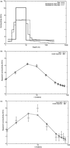
Results are presented in Figure 1 for synthetic data. The obtained model for the original data is shown n Figure 1(a) and fitness to data in 1(b). RMS fitness is 0.88 for data of Figure 1(b) with errors σ = 0.1 and λ = 1. It can be observed that the model obtained has sharp discontinuities near the true locations. The fact they are not exactly where they should be is not a drawback of the inversion method, but a product of the well-known phenomena of equivalence. Two conductive layers are equivalent if they have the same conductivity-thickness product, as in the present case. Physically, this happens because both have approximately the same capability to carry inductive currents and to produce magnetic effects at the receiver. The original data obtained of the synthetic model presented before were contaminated by adding Gaussian noise (mean zero, standard deviation (sd) 0.5) in order to observe the effect on the resulting model. Figure 1 also presents the model developed for the noisy data with λ = 1, σ = 0.5, and the fitness (RMS=0.9) is observed on Figure 1(c). From those figures it can be observed that the model structure remains recovered under that noise contamination of data.

Figure 1. (a) Developed models and fitness to (b) original and (c) noise contaminated data for a synthetic three-layer model. The data correspond to apparent conductivity measurements for a vertical coil configuration with multiple separations.

The previous example leads naturally to a linear integral equation for the unknown model m(z). In general, geophysical inverse problems are nonlinear. In what follows, we consider two cases: direct-current resistivity and magnetotelluric soundings 22,23. Direct-current resistivity soundings are obtained using electrodes placed on the surface of the ground at different separations. Direct current is injected to the ground by means of two outer electrodes, and voltage is measured between two inner electrodes. Voltage measurements are taken for multiple separations of the outer electrodes and expressed as apparent resistivity. Typical separations are of a few meters for the inner pair and of several hundred meters for the outer pair, the longer the separation the greater the depth of penetration. The recovery of the vertical resistivity profile is a plausible goal provided there are data for multiple separations. The model is a multilayer structure changing over depth (z), overlaying a half-space. Every element of the model (m_j) would consist of the resistivity of i-th layer. The relationship among measurements and resistivities of a layered medium is also modelled by an integral equation, but now with a nonlinear kernel. The forward equation for this model is given by 22where r_i is half the separation of the outer electrodes. J₁ denotes the Bessel function of order one and μ the integration variable. Resistivity transform function for a layered media is represented by the recurrence equationwith n the number of layers and ρ_i and t_i the resistivity and thickness of i-th layer, respectively.

In the inversion algorithm we simulate an arbitrary variation of resistivity with depth by dividing the ground into many thin layers whose resistivities represent the model m(z). The thicknesses of the layers are kept constant.

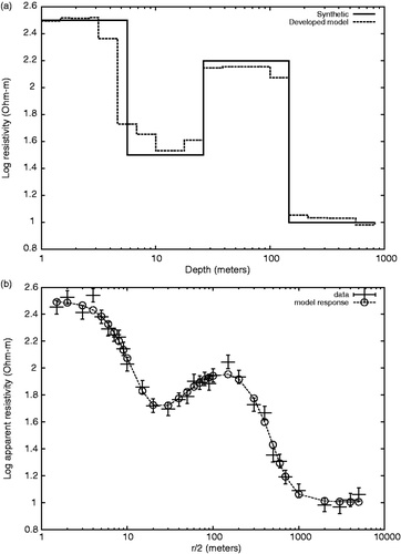
Figure 2 presents a developed model for synthetic data obtained from a four-layer model for a λ = 200, obtaining a RMS fitness of 1.0 also considering errors σ = 0.01. To observe the results of noise degradation on data, Gaussian noise (mean zero, sd = 0.05) was added to the synthetic data produced by model of Figure 2. In Figure 3, the resulting model is presented, observing that it is practically the same as obtained for the original noise-free data. The data is presented with error bars the size of σ.

Figure 2. (a) Developed model and (b) fitness to synthetic data for a four layered synthetic model in the DC geosounding method.

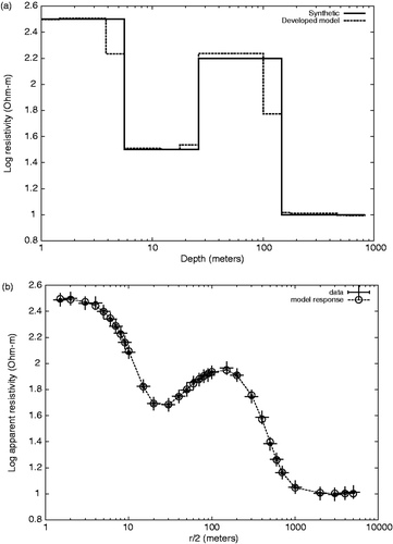
Figure 3. (a) Developed model and (b) fitness for synthetic model in Figure 2 when Gaussian noise (μ = 0, sd = 0.05) is added to data.

We now turn to the case of magnetotelluric soundings. They are deep soundings that are obtained using naturally occurring electric and magnetic fields that originate in the ionosphere. In this case, what determines the depth of penetration is not the separation between source and receiver, which is fixed by nature, but the frequency or period of the fields. Typical periods range from less than a second to several thousands of seconds, and the corresponding depths of penetration from tens of meters to tens of kilometers. In this case, there are two sounding curves: one of apparent resistivity versus period, and the other the phase of the electric field with respect to the magnetic field, again versus period. The recovery of the vertical resistivity profile is plausible provided there are data for multiple periods.

The inverse MT problem aims to the reconstruction of ρ(z) from the parametric dependence of the impedance Z(z = 0, ω) upon the angular frequency ω. From Z, the apparent resistivity ρ_a is defined as , and the phase . The data d_i = {ρ_a, φ}_i consist of measurements of apparent resistivity and phase at a given frequency ω_i (period T_i). The impedance at the surface is given by the recurrent equation 24with , e_j = exp(−2γ_jh_j), layer thickness h_j, and for the terminating half-space . Again, in the inversion algorithm, we simulate an arbitrary variation of resistivity with depth by dividing the ground into many thin layers whose resistivities represent the model m(z). The thicknesses of the layers are kept constant.

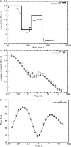
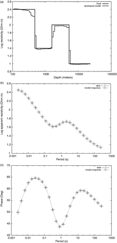
In Figure 4, the model obtained for synthetic data for a three-layer model is presented, using λ = 400 with a RMS fitness of 1.0 considering equal errors σ = 0.01.

Figure 4. Developed model (a) and data fitness (magnitude (b) and phase (c)) from a four-layered synthetic model for the MT geosounding method.

As in the previous case, Gaussian noise is added to the data to observe effects on model deterioration. Figure 5 presents a developed model for the same synthetic data obtained from the layered model in Figure 4, but now adding Gaussian noise (mean zero, sd = 0.05 for apparent resistivity and sd = 0.5 for phase), obtaining a RMS fitness of 1.0 with λ = 40. The observed model suffer some changes, but discontinuities remain on same locations; essentially the model has the same structure as the one obtained for the original data. From those results, it can be noticed how the discontinuities are enhanced when the l₁ term is enforced after α = 1.

Figure 5. Developed model (a) and data fitness (magnitude (b) and phase (c)) for the synthetic model presented on Figure 4 when Gaussian noise (μ = 0, sd = 0.05 for apparent resistivity and sd = 0.5 for phase) is added to data.

5. Application to real data

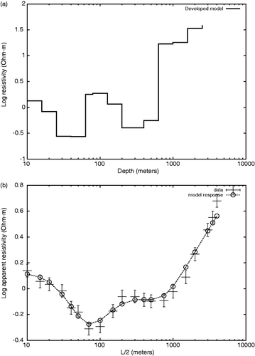
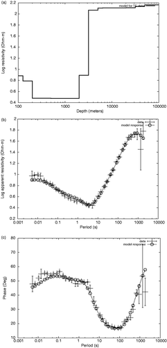
To illustrate the performance of the algorithm to real, field data, we chose to apply it to magnetotelluric site PCS0012 of COPROD2 data set 25. This is a dataset of 35 magnetotelluric sites effected on southern Saskatchewan and Manitoba, Canada. The data were acquired in 1984 and 1985 by Phoenix Geophysics Ltd. of Toronto, for PanCanadian Petroleum Ltd. The 400 Km east-west profile crosses hydrocarbon-rich Willinston basin, and, within the basement, the North American Central Plains (NACP) conductivity anomaly. This site is on the western end of the profile, far from the NACP anomaly. The developed model, along with the data responses are presented in Figure 6. Observe the great variances on some data. The data has been studied by several researchers 25 who considered subsets of them, in the period range of [10, 1000] and reducing the error range. All of the original measurements for this site were applied to the algorithm, with λ = 400 and stopping when fitness was RMS = 2.9. The misfit to the data, larger than the desired of RMS=1.0, is biased towards short periods. This means that a one-dimensional model is not entirely adequate for shallow depths of the order of 100 meters. However, it can be observed that for the rest of the periods the response of the model follows the data within the experimental uncertainties. The recovered structure is observed in several models presented on COPROD2 report, 25 particularly those named ‘jones1’ and ‘jones2’ originally presented on 26.

Figure 6. Developed model (a) and data fitness (magnitude (b) and phase (c)) for site PCS012 of COPROD2 MT data set.

We also applied the algorithm to a real direct-current resistivity sounding. The data corresponds to site 25 of line 1 of an extensive survey 27 effected by Comisión Federal de Electricidad from Mexico and Lawrence Berkeley Laboratory of University of California, Berkeley. The Cerro Prieto geothermal reservoir is located on Mexicali, Mexico, and is home of Cerro Prieto Geothermal Power Station, which now produces 720 MW of electrical power. The chosen sounding has unusually long source-receiver separations of 10 km (r = 5 km). The final model is shown in Figure 7. A relative error sd = 0.05 was assumed for the data. The response of the final model is compared with the field data shown in Figure 7(b). The program was stopped when RMS = 0.84 with λ = 2. The recovered vertical structure is very similar to that obtained by Wilt et al. 28 who used a 2-D modelling program in the interpretation of the complete survey.

Figure 7. Developed model (a) and data fitness (b) for site 25 of line 1 in Cerro Prieto data set.

6. Conclusions

A hybrid inversion algorithm is proposed for a non-separable regularization operator. The algorithm is based on a homotopy moving from a l₂ to a l₁ regularization operator and implemented by coordinate descent. Results are presented for synthetic data of electromagnetic, direct-current and magnetotelluric sounding methods. The developed models recover the blocky structure of the model used to generate the data, even under noise contamination of the data. Results are also presented for field data obtaining models comparable with those presented elsewhere.

Acknowledgements

The authors would like to acknowledge F. Arellano from Comisión Federal de Electricidad, México, for making the Cerro Prieto data available.

References

- Tikhonov, A, and Arsenin, VY, 1977. Solutions of Ill-Posed Problems. Washington, DC: V.H. Winston & Sons; 1977.
- Parker, R, 1994. Geophysical Inverse Theory. Princeton, NJ: Princeton University Press; 1994.
- Constable, SC, Parker, RL, and Constable, CG, 1987. Occam's inversion: A practical algorithm for generating smooth models from electromagnetic sounding data, Geophysics 52 (1987), pp. 289–300.
- Hidalgo, H, Marroquín, JL, and Gómez-Treviño, E, 1998. Piecewise smooth models for electromagnetic inverse problems, IEEE Trans. Geosci. Remote Sens. 36 (1998), pp. 556–561.
- Esparza, FJ, and Gómez-Treviño, E, 1987. Electromagnetic sounding in the resistive limit and the Backus–Gilbert method for estimating averages, Geoexploration 24 (1987), pp. 441–454.
- Dobson, D, 1997. "Recovery of blocky images in electrical impedance tomography". In: Engl, HW, and Rundell, W, eds. Inverse Problems in Medical Imaging and Nondestructive Testing. New York: Springer; 1997. pp. 43–64.
- Vogel, C, and Oman, M, 1998. Fast, robust total variation-based reconstruction of noisy, blurred images, IEEE Trans. Image Process. 7 (1998), pp. 813–824.
- Vogel, CR, 2002. Computational Methods for Inverse Problems. Philadelphia, PA: SIAM Frontiers in Applied Mathematics; 2002.
- Chan, T, Esedoglu, S, Park, F, and Yip, A, 2006. "Recent developments in total variation restoration". In: Paragio, N, and Faugeras, O, eds. Handbook of Mathematical Models in Computer Vision. New York: Springer; 2006. pp. 17–32.
- Nashed, MZ, and Scherzer, O, 1998. Least squares and bounded variation regularization with nondifferentiable functionals, Numer. Funct. Anal. Optim. 19 (1998), pp. 873–901.
- Friedman, J, Hastie, T, Hoefling, H, and Tibshirani, R, 2007. Pathwise coordinate optimization, Ann. Appl. Stat. 1 (2007), pp. 302–332.
- Tibshirani, R, 1996. Regression shrinkage and selection via the lasso, J. R. Stat. Soc. Ser. B 58 (1996), pp. 267–288.
- Efron, B, Hastie, T, Johnstone, I, and Tibshirani, R, 2004. Least angle regression, Ann. Stat. 2 (2004), pp. 407–499.
- Hidalgo, H, Gómez, E, and Pérez, MA, 2004. Linear programs for the reconstruction of 2D images from geophysical electromagnetic measurements, Subsurface Sens. Technol. Appl. 5 (2004), pp. 79–96.
- Osborne, MR, Presnell, B, and Turlach, BA, 2000. A new approach for variable selection in least squares problems, IMA J. Numer. Anal. 20 (2000), pp. 389–404.
- Tseng, P, and Yun, S, 2009. A coordinate descent method for nonsmooth separable minimization, Math. Program. Ser. B 117 (2009), pp. 387–423.
- Zou, H, and Hastie, T, 2005. Regularization and variable selection via the elastic net, J. R. Stat. Soc. Ser. B 67 (2005), pp. 301–320, Part 2.
- Wang, Y, Cui, Y, and Yang, C, 2011. Hybrid regularization methods for seismic reflectivity inversion, Int. J. Geomath. 2 (2011), pp. 87–112.
- Ito, K, and Kunisch, K, 2000. Augmented Lagrangian methods for nonsmooth, convex optimization in Hilbert spaces, Nonlinear Anal. 41 (2000), pp. 591–616.
- D.M. Malioutov, M. Cetin, and A.S. Willsky, Homotopy continuation for sparse signal representation, IEEE International Conference on Acoustics, Speech, and Signal Processing, Montreal, Canada, 2005.
- Gómez-Treviño, E, Esparza, F, and Méndez-Delgado, S, 2002. New theoretical and practical aspects of electromagnetic soundings at low induction numbers, Geophysics 67 (2002), pp. 1441–1451.
- Koefoed, O, 1979. Geosounding Principles, 1 Resistivity Sounding Measurements. Amsterdam: Elsevier Scientific Pub. Co.; 1979.
- Simpson, F, and Bahr, K, 2005. Practical Magnetotellurics. Cambridge: Cambridge University Press; 2005.
- Meju, M, 1994. Geophysical Data Analysis: Understanding Inverse Problem Theory and Practice. Vol. 6. Tulsa, OK: Society of Exploration Geophysicists; 1994, Course Notes Series.
- Jones, A, 1993. The Coprod2 Dataset: Tectonic Setting, Recorded MT Data, and Comparison of Models, J. Geomag. Geoelectr. 45 (1993), pp. 933–955.
- Jones, A, and Craven, JA, 1990. The North American Central Plains conductivity anomaly and its correlation with gravity, magnetics, seismic, and heat flow data in the Province of Saskatchewan, Phys. Earth Planet. Inter. 60 (1990), pp. 169–194.
- Razo, A, Arellano, F, and Fonseca, H, 1978. "Estudios de resistividad realizados por CFE en Cerro Prieto". In: Proceedings of the First Symposium on the Cerro Prieto Geothermal Field. Baja California, Mexico, San Diego, CA. 1978.
- Wilt, MJ, Goldstein, NE, and Razo, A, 1978. "LBL resistivity studies at Cerro Prieto". In: Proceedings of the First Symposium on the Cerro Prieto Geothermal Field. Baja California, Mexico, San Diego, CA. 1978.