Conductivity reconstructions using real data from a new planar electrical impedance tomography device

Abstract

In this paper, we present results of reconstructions using real data from a new planar electrical impedance tomography device developed at the Institut für Physik, Johannes Gutenberg Universität, Mainz, Germany. The prototype consists of a planar sensing head of circular geometry, and it was designed mainly for breast cancer detection. There are 12 large outer electrodes arranged on a ring of radius  cm where the external currents are injected, and a set of 54 point-like high-impedance inner electrodes where the induced voltages are measured. Two direct (i.e. non-iterative) reconstruction algorithms are considered: one is based on a discrete resistor model, and the other one is an integral equation approach for smooth conductivity distributions.

Keywords:

• electrical impedance tomography
• integral equation methods
• resistor networks
• breast cancer detection
• nonlinear inverse problems
• ill-posed problems

Classification:

• 31B10
• 45Q05
• 47A52
• 65F20
• 65F22

Introduction

Electrical impedance tomography (EIT) is a noninvasive, portable, low-cost technology developed to image the electrical conductivity distribution within an object from boundary measurements of the electric currents and voltages. Since different materials display different electrical properties, EIT can be used as a method of industrial, geophysical and medical imaging [1]. One of the possible medical applications is breast cancer detection [2–11].

Breast cancer is presently routinely detected by palpation, X-ray mammography and ultrasound imaging with sensitivity rates of up to 90%. These classical diagnostic methods, however, yield rather unspecific results. Only one in five biopsies of suspicious lesions leads to a malignant histological diagnosis [12]. Research is therefore aimed at developing alternative imaging techniques to diagnose breast cancer more accurately and possibly earlier. Since in vivo studies discovered a difference of three times or more in the specific electrical conductivity between healthy and cancerous tissue [13–15], imaging the electrical properties of breast tissues would yield important information which can improve the specificity of the diagnosis. Electric impedance mammography (EIM) may therefore be used as an aid to detect breast cancer in its earliest stages of development (as an adjunct to or a replacement for traditional X-ray tomography). However, EIM has not yet made the transition from an exciting medical physics discipline into widespread routine clinical use. The issues are both theoretical: the inverse conductivity problem is mathematically challenging being both nonlinear and extremely ill-posed in the Hadamard sense and it has poor spatial resolution [16], and practical: errors in the electrode position and boundary shape, high and uncontrollable skin-electrode contact impedance. The variations in the contact impedance are often up to 20 or more, and the errors in the current densities and measured voltages are often larger than the effect of inhomogeneities in the interior of the body.

The latest EIT device developed at the Institut für Physik, Johannes Gutenberg Universität, Mainz, Germany, is in some aspects similar to those described in [2–6, 9, 17–19]. Note, however, that the T-Scan technology [2, 4] does not produce tomographic reconstructions, it just maps the surface impedance using 256 electrodes. The Mainz EIT device consists of a planar sensing head of circular geometry, and it was designed mainly for breast cancer detection. There are 12 large outer (active) electrodes arranged on a ring of radius  cm where the external currents are injected, and a set of 54 point-like high-impedance inner (passive) electrodes where the induced voltages are measured. To avoid any problems due to the unknown contact impedance, the voltages are not measured at the outer (active) electrodes. At the inner (passive) electrodes, very high impedance voltage measurements are taken, and the problem of the contact impedance does not arise. The voltage measurements are relative to the system’s ground. Further developments in the electronics of the device are planned to allow measurements of electrode-electrode potential differences. Almost all previous EIT devices use the same electrodes for current injection and voltage measurement. The excitation current is injected (extracted) at one pair of electrodes at each time and the resulting voltage is measured at all or some of the remaining electrodes, e.g. [5, 6]. In this way, the problem with the high and uncontrollable skin-electrode contact impedance is avoided but at the price of aggravating the ill-posedness of the reconstruction. The novelty of the device, and hence of the reconstruction methods proposed, consists exactly in the distinct use of active and passive electrodes. The active electrodes are used only for current injection while the passive electrodes only for voltage measurements. The device has a fixed geometry, the positions of the electrodes are exactly known and there are no issues related to the contact impedance.

The EI imaging technique proposed in this paper may be used as a low-cost, portable medical screening method or as an aid to detect breast cancer in its earliest stages of development as an adjunct to other traditional imaging techniques. Since the EIT device is much smaller than the human body to which it is applied, the imaging of the conductivity distribution of the three-dimensional half space might be required from electrical measurements performed on its surface. Many reconstruction procedures addressing the full three-dimensional nonlinear inverse conductivity problem have been developed, e.g. [17, 20, 21]. However, these procedures can be quite demanding computationally, slowly convergent or quite sensitive to numerical or data errors. These concerns have encouraged the search for reconstruction algorithms which reduce the computational demands either by using some a priori information or by developing non-iterative procedures. If a tumour is situated at a shallow depth, a map of the conductivity at the surface of the skin provides enough information on the existence and location of the tumour. Hence, we determine the conductivity of a two-dimensional circular domain from boundary measurements of currents and interior measurements of the potential. The inverse problem to solve is different from the classical inverse conductivity problem, and the ill-posedness is circumvented to a certain extent. Two non-iterative reconstruction algorithms for this inverse problem were presented in [19]: one is based on a resistor network model and the other on reformulating the problem in terms of integral equations. The numerical reconstructions from simulated data had very good spatial resolution, and the algorithms seemed to be quite robust with respect to errors in the data in general, and to errors in the input currents in particular. It is important to mention that the map of the conductivity at the surface can be used as valuable a priori knowledge to create a model conductivity distribution as a first estimate of the solution if our non-iterative inversion techniques are extended to address the full three-dimensional problem in order to obtain additional information about the depths of the tumours.

In this paper, we present the conductivity reconstructions from tank phantom data. A detailed description of the Mainz tomograph and of the experimental set-up used for data collection is given in Section 2. In Section 3, the mathematical setting is presented and the two reconstruction algorithms are briefly reviewed. Section 4 contains a selection of numerical reconstructions obtained from real data.

Description of the device

The Mainz tomograph consists of three parts: an electronic device to generate well-defined current patterns and measure electric potentials, a sensing head, and a computer for the image reconstruction, see Figure 1.

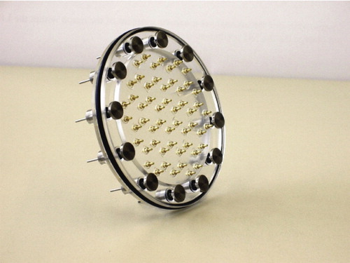
The sensing head has a diameter of 10 cm and consists of 12 large electrodes, arranged on the outer ring of a disk of radius  cm where the external currents are injected, and a set of 54 small high-impedance inner electrodes placed on a hexagonal pattern in the interior which are used to measure the voltages, see Figure 2.

The data acquisition device consists of five modules (cf. Figure 3). The first module is a micro controller to facilitate the communication between the measuring device and external components via a RS232 serial interface. The second module generates pre-set sinusoidal voltages of frequency  kHz which can be used to drive current injecting electrodes. The amplitudes can be modulated with 16-bit accuracy to any desired amplitude pattern by 32 ADCs. The resulting current at each injection electrode passes through a precision resistor and a special operational amplifier to facilitate the measurement of the current. The voltages on the interior electrodes are measured with 16-bit accuracy with the help of the third module. The fourth module serves to read the data and to measure the signal by a peak detector largely in parallel via 8 multiplexers of 16 channels each. The measured value of the peak detector is subsequently digitalized to 16-bit accuracy. In the fifth module, finally, the sign of the modulation is defined.

Fig. 1 The Mainz tomograph.

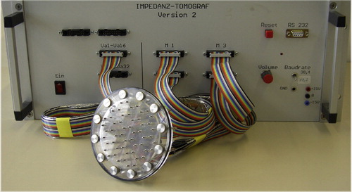
Fig. 2 The sensing head.

There are independent measurements for current injecting electrodes. In most reconstruction algorithms, it is assumed that currents are prescribed and voltages are measured. Because of the much simpler electronic implementation, we apply voltages on the injectors and measure the corresponding currents. It is, however, no problem to convert to current-driven data by linear combination of the various voltage-driven data. Standard trigonometric voltages or current patterns of different spatial frequencies are applied at the outer electrodes [22]. At the interior high-resistance electrodes, only voltages are measured.

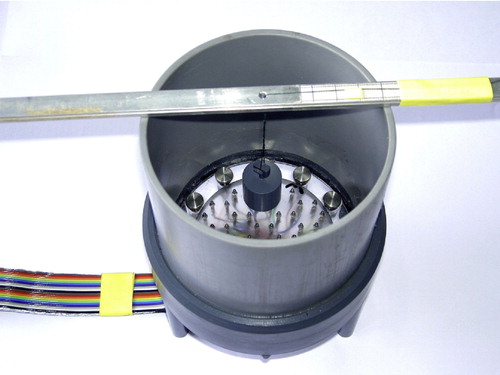
The tomograph is designed primarily for mammography. So far, however, we have no clinical data at our disposal. Instead, we have placed the sensing head at the bottom of two cylindrical tanks, a small one of the same diameter as the sensing head and a large one of a much larger diameter. Both tanks were filled with a conducting liquid (salt water). Cylindrical metallic objects of various diameters and a cubic agar phantom were immersed in the liquid at different distances from the sensing head, see Figure 4. In this paper, we present the conductivity reconstructions obtained from real data which were obtained in this way.

Fig. 3 The data acquisition device.

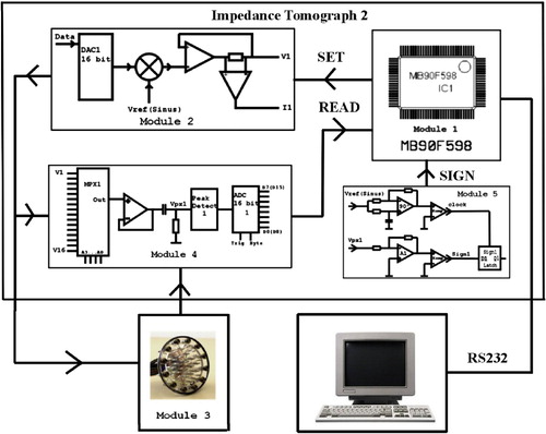
Fig. 4 Experimental setup.

Mathematical formulation and reconstruction algorithms

Mathematical setting

Let , and be an isotropic conductivity distribution in . If there are no internal current sources in , for an applied current density , the electric potential satisfies the following elliptic partial differential equation(1) subject to Neumann boundary conditions(2) The boundary value problems (1) and (2) has a unique solution up to an additive constant, which we could fix by choosing the ground either as(3) (4) The inverse problem under consideration can be formulated mathematically as follows: find the conductivity function in satisfying (1)–(3) or (1), (2) and (4) from the measurement operator(5) where .

Remark 1.

Let . If for any , the solution of the Neumann boundary value problems (1)–(3), , is known then by standard trace theorems is known. Hence, we have a full knowledge of the Neumann to Dirichlet map, and can be uniquely reconstructed [23].

Remark 2.

Let be the solution of the Neumann boundary value problems (1)–(3) for a given . If is non-constant in , and the conductivity is known and is sufficiently smooth (in particular continuous), then can be uniquely extended to a Lipschitz continuous (admissible) function in [24].

In practice, however, we only have partial and noisy knowledge of the measurement operator . Only 10 standard varying-frequency patterns of the input current are applied on :(6) and we can only measure the potential at 54 points:(7) Moreover, in practice, we do not know the current densities for all . What we actually know are the currents sent along wires which are attached to the 12 outer discrete electrodes. Since in the usual EIT set-ups the voltages are measured at the same electrodes used for current injection, the effects of the contact impedance need to be taken into account and the modelling of the current flow through the electrodes is of utmost importance. However, since in our experimental set-up the voltages are not measured at the outer electrodes, a continuum (no electrode) model is used for the integral equation method while the resistor network approach uses a perfectly conducting electrode model. More information about electrode models can be found in [25, 26].

Integral equation reconstruction method

Let us consider that is the reference or background conductivity. The associated potential is the solution of the boundary value problems (1)–(3) for , namely(8) where is the Neumann Green’s function for the Laplace equation in the disk [27].

If is smooth and strictly positive, Equation (1) can be rewritten as(9) If we assume that near , the solution of problems (1)–(3) is(10) Furthermore, it was shown in [19] that if , a partial integration in (8) leads to the following integral equation for :(11) where is known in .

Since, in practice, we only have partial knowledge of the measurement operator in (5), Equation () reduces to a system of integral equation for :(12) where are the integration kernels, and the reference potentials for the input currents (10) are explicitly known:(13) In order to find , we discretize the system of equations (9) as follows:(14) where are the polar coordinates of the interior points of measurements, and is a set of quadrature weights and points for the disk of radius given by Engels [28]. The above system of equations is over-determined (540 equations for 172 unknowns) and it is solved by means of the generalized inverse. Truncated singular value decomposition is used as regularization scheme [29]. In this way, very small singular values (i.e. smaller than ) will be cut out and will not enter in the reconstruction. More details can be found in [19].

Resistor network model

A simpler reconstruction algorithm can be obtained if we model the measurement area as a resistor network. The model consists of hexagonal resistance patterns as shown in Figure 5.

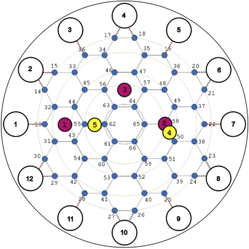
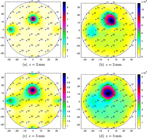
Fig. 5 Layout of the electrode array of the Mainz EIT device. The small circles labelled from 1 to 12 show the outer electrodes for current injection. The position of the 54 inner electrodes for potential measurements are drawn as thick points (marked in blue). The network is used as a model of the measurement area. The positions 1, 2 and 3 (marked in red) indicate the places above the sensing head where metallic objects were immersed in conducting liquid for the experimental set-up described in Figure 4, while the positions 4 and 5 (marked in yellow) indicate the places where an agar phantom was placed.

In EIT, the reconstruction of conductances in resistor networks from full or partial knowledge of the Neumann-to-Dirichlet map as well as the design of adaptive optimal grids attracted considerable research interest over the years [22, 30–35]. However, the inverse problem considered in this paper is different from the classical inverse conductivity problem: find the conductances assigned to each link in the network from measurements of currents at the boundary knots and measurements of the potential at the inner knots. Although rather simple, the network consisting of hexagonal resistor patterns which models the measurement area enables us to design a non-iterative inversion algorithm and hence, as shown below, to determine the conductances in the grid in a straightforward way.

Fig. 6 Conductivity reconstructions from reference data (small tank filled with salt water and no immersed objects) : (a) using the integral equation approach and (b) using the resistor network approach.

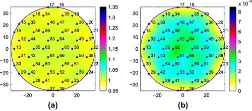
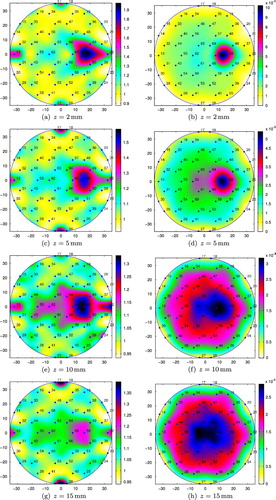
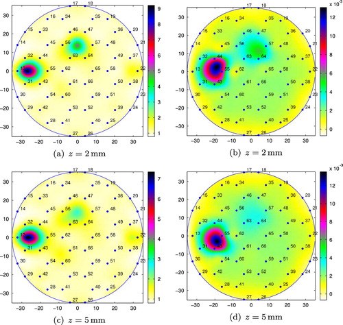
Fig. 7 Conductivity reconstructions for M20 placed at position 1 (small tank): (a), (c) and (e) using the integral equation approach; (b), (d) and (f) using the resistor network approach.

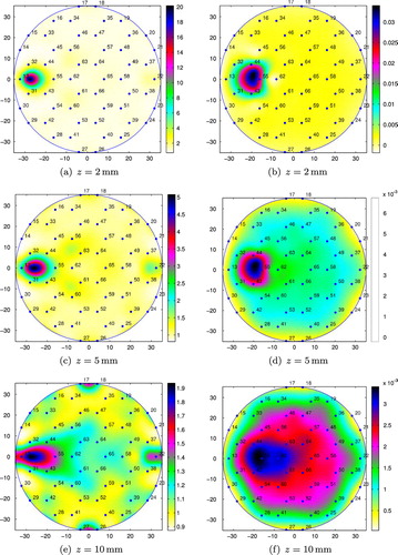
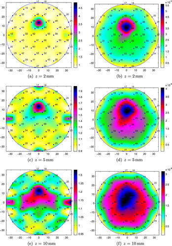
Fig. 8 Conductivity reconstructions for M15 placed at position 1 (small tank): (a), (c), and (e) using the integral equation approach; (b), (d), and (f) using the resistor network approach.

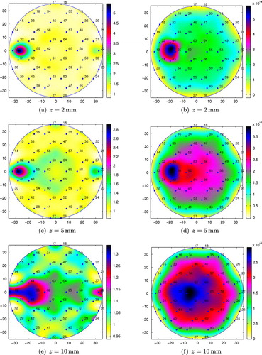
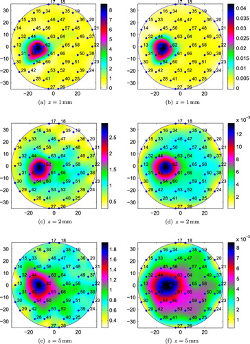
Fig. 9 Conductivity reconstructions for M15 placed at position 2 (small tank): (a), (c), (e) and (g) using the integral equation approach; (b), (d), (f) and (h) using the resistor network approach.

The effective resistance network consists of knots where the potentials are measured and links () connecting the knots and . Let be the current flowing from knot to knot , be the resistance of the link and be the corresponding conductance. We introduce a compound index to enumerate the linksan -dimensional vector of conductances assigned to the links, and a dimensional matrix of potential differences whose elements are defined byAs shown in [19], Kirchhoff’s first law (current conservation) combined with Ohm’s law gives(15) where(16) A subtle point is the way in which the current splits up into two components at 6 of the 12 current injectors which do not lie directly next to the neighboring inner voltage electrodes. The splitting ratios are calculated from synthetic data for a constant conductivity. We have shown in [19] that the results of the reconstruction are largely insensitive to this assumption. Once this assumption has been made, the 12 external electrodes and the outer layer of resistances (dashed lines in Figure 5) do not need to be included in the network any longer. There are now effective currents entering the network in the second outermost layer. Hence, for are the effective external applied currents, and for . Equation () represents a linear system of equations for the unknown conductances , . Because of current conservation, only equations are linearly independent, and the system of equations () is underdetermined. In order to obtain a solution of this system of equations, we add information from repeated measurements with different patterns of injected currents (10), i.e.(17) where , , is the angular position of the external current electrodes. Hence, an over-determined system is obtained which can be solved conveniently by generalized inversion and the singular value decomposition.

Fig. 10 Conductivity reconstructions for M15 placed at position 3 (small tank): (a), (c) and (e) using the integral equation approach; (b), (d) and (f) using the resistor network approach.

Numerical reconstructions from real data

The numerical experiments with simulated data in [19] showed that the two inversion techniques proposed in Section 3 reconstruct the positions and the sizes of both high and low conductivity regions. However, for mammography, we are only interested in detecting high conductivity regions.

Fig. 11 Conductivity reconstructions for M15 placed at position 3 (large tank): (a), (c) and (e) using the integral equation approach; (b), (d) and (f) using the resistor network approach.

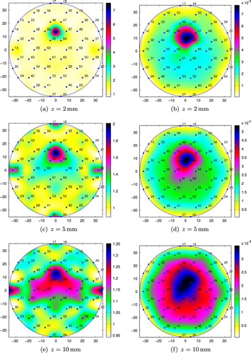
Fig. 12 Conductivity reconstructions for M15 placed at position 1 and M20 placed at position 3 (small tank): (a) and (c) using the integral equation approach; (b) and (d) using the resistor network approach.

The first set of numerical reconstructions presented in this section are for two cylindrical metallic objects, M20 and M15, which have diameters and heights equal to 15 and 20 mm, respectively. The objects were immersed in conducting liquids (salt water) at various distances from the sensing head and placed either at a position in between the inner electrodes, position 1 or 3 in Figure 5 or on the top of an inner electrode, position 2 in Figure 5. The water level in the tank was approximately 8 cm. It is important to remark that although the distances were accurately measured, for technical reasons, the actual positions of the immersed objects might differ slightly from those indicated in Figure 5. As mentioned in subsection Section23.3, the inner electrodes where the voltages are measured are placed in a hexagonal pattern. All hexagons marked in Figure 5 are regular with side length of 8.1 mm. Hence, the sizes of the objects used are smaller or larger relative to the sizes of these hexagons, i.e. M15 and M20 have smaller and larger radii, respectively, than the side of the hexagons. The numerical results for both objects should therefore be considered. The detection of M15 (which covers no electrodes in positions 1 and 3, and only one electrode in position 2) tests the spatial resolution of our inversions, while the reconstructions for M20 which covers more electrodes (six in positions 1 and 3 and four in position 2) test the sensitivity of the algorithms.

Fig. 13 Conductivity reconstructions for M20 placed at position 1 and M15 placed at position 3 (small tank): (a) and (c) using the integral equation approach; (b) and (d) using the resistor network approach.

The inversion algorithm for the integral equation approach was described in subsection Section23.1. Although the conductivity distribution is assumed to be smooth, in order to find , the system of integral equations (9) needs to be discretized. Hence, the values of the conductivity at 172 inner points are obtained by inverting the over-determined linear system of equations (11). In the numerical examples considered, singular values smaller than were cut off (i.e. 24 singular values were used in the reconstructions). Using the reconstruction algorithm for the resistor network described in subsection Section23.3, the values of the conductivity at 72 inner points (i.e. mid-points of the resistor network links) are obtained. In order to find the values of the conductivity at any point inside the disk of radius 4.8 cm, we used in both approaches the Matlab 4 griddata interpolation method. Therefore, the quality of the reconstructions depends both on the number of discretization points and on the accuracy of the Matlab interpolation routine which were used.

Note that in all figures presented below the colour ranges are different for each subplot. The resistor network reconstructs absolute conductivities, while the integral equation algorithm reconstructs conductivities relative to the reference background conductivity . However, in both reconstruction techniques, only absolute data were used (i.e. we do not use in our reconstructions the measurements of the reference potentials corresponding to a tank with no objects immersed). For the integral equation approach, if the background conductivity is known then an estimate of the actual conductivity distribution could be obtained by multiplying the reconstructed values by . The results obtained from the two algorithms are comparable. The homogeneity properties of the two proposed algorithms are good as it can be seen from Figure 6 which shows the conductivity reconstructions obtained from the data for the small tank filled with salted water only.

In Figure 7, we present the conductivity reconstructions for the metallic object M20, immersed in salt water in the small tank at distances , 5 and 10 mm from the sensing head, and placed at position 1. The numerical results for the smaller metallic object, M15, placed at positions 1, 2 and 3 can be found in Figures 8,9 and 10, respectively. The metallic objects could still be detected up to distances from the sensing head which are approximately equal to their diameters (e.g. see Figure 9(g)), and it does not matter whether the objects are placed on a position in between the inner electrodes, position 1 or position 3, or on the top of an inner electrode, position 2. The integral equation method seems to be able to better detect objects situated at larger distances from the sensing head than the resistor network approach.

Fig. 14 Conductivity reconstructions for a cubic agar phantom placed at position 4 (small tank): (a), (c) and (e) using the integral equation approach; (b), (d) and (f) using the resistor network approach.

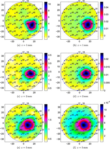
Fig. 15 Conductivity reconstructions for a cubic agar phantom placed at position 5 (small tank): (a), (c) and (e) using the integral equation approach; (b), (d) and (f) using the resistor network approach.

One of the assumptions we used in our inverse problem formulation was that the current flowing outside the domain is unimportant. In order to test the validity of this assumption, we compared the conductivity reconstructions from data obtained from the small tank and the large one, see Figures 10 and 11. There is no significant difference in these reconstructions which therefore supports our hypothesis.

The reconstructions obtained for both metallic objects, M20 and M15, immersed in the small tank at the same distances from the sensing head are shown in Figures 12 and 13. The presence of the small metallic object, M15, is slightly shielded by the larger object, M20.

In order to show that it is possible to detect not only metallic objects but also lower contrast inclusions, we also performed experiments with a cubic agar phantom of side equal to 20 mm. The agar phantom was immersed in the small tank filled with salt water and placed at positions 4 and 5 (see Figure 5) and at distances and 5 mm from the sensing head. Although both position 4 and position 5 are in between two neighbour inner electrodes, the agar phantom covers six electrodes in position 5 and only two electrodes in position 4. Figures 14 and 15 present the conductivity reconstructions for the agar phantom.

The approach based on the resistor network model reconstructs directly the absolute values of the conductivity, while the integral equation method seems to be able to detect objects situated at larger distances from the sensing head especially if they are relatively large (for the considered geometry, of radius larger than the side of a hexagon).

Conclusion

In this paper, we have presented conductivity reconstructions from real data obtained from a new planar EIT device intended for breast cancer detection. A map of the conductivity at the surface to which the device is applied could provide some valuable information on the existence, location and size of breast tumours situated at shallow depths. Hence, we have attempted to reconstruct the conductivity of a two-dimensional circular domain from boundary measurements of currents and interior measurements of the potential. For our experiments, the sensing head of our device was placed at the bottom of two tanks of different diameters filled with salt water of various concentrations. One or two metal objects of different sizes and a cubic agar phantom were placed inside the liquid at different distances from the sensing head. Two inversion techniques have been used: the first one is an integral equation approach for smooth conductivity distributions, while the second one is based on a discrete resistor model. With both methods, the positions of the metallic objects could be detected up to distances from the sensing head which are approximately equal to their diameters. These are promising first results, but there still remains significant clinical testing to determine whether this device and the proposed algorithms will prove effective for breast cancer detection.

The two reconstruction techniques that we have used are based on a very different modelling of the measurement area and both algorithms lead, in general, to quite similar reconstructed images. A combination of the complementary reconstruction algorithms should help us to further improve the robustness of our method.

We are currently trying to improve the electronics of the EIT device in order to measure the voltages at the inner electrodes even more accurately. This will enable us to detect much deeper objects. Increasing the number of inner electrodes where voltages are measured and/or imposing sparsity constraints on the conductivity could improve greatly the quality of reconstructions. We also plan to extend our techniques to a fully three-dimensional model of the problem in order to obtain additional information about the depths of the tumours. Further studies on the accuracy of the locations of the detected inclusions, and on the dependence of the conductivity distributions of these inhomogeneities on the distance from the sensing head, are likely to provide very useful a priori information for the three-dimensional inversion techniques.

Acknowledgments

This work has been partially supported by the German Federal Ministry of Education and Research (BMBF) under the Grant 03SCPAM3.

References

- Borcea, L, 2002. Electrical impedance tomography, Inverse Probl. 18 (2002), pp. R99–R136.
- Laver-Moskovitz, O, 1996. T-Scan: A New Imaging Method for Breast Cancer Detection without X-ray. Chicago, IL: RSNA Presentation; 1996.
- Perlet, C, Kessler, M, Lenington, S, Sittek, H, and Reiser, M, 2000. Electrical impedance measurement of the breast: effect of hormonal changes associated with the menstrual cycle, Eur. Radiol. 10 (2000), pp. 1550–1554.
- Assenheimer, M, Laver-Moskovitz, O, Malonek, D, Manor, D, Nahliel, U, Nitzan, R, and Saad, A, 2001. The T-scan technology: electrical impedance as a diagnostic tool for breast cancer detection, Physiol. Meas. 22 (2001), pp. 1–8.
- Cherepenin, V, Karpov, A, Korjenevsky, A, Kornienko, V, Mazaletskaya, A, Mazourov, D, and Meister, D, 2001. A 3D electrical impedance tomography (EIT) system for breast cancer detection, Physiol. Meas. 22 (9) (2001), pp. 9–18.
- Cherepenin, VA, Karpov, AY, Korjenevsky, AV, Kornienko, VN, Kultiasov, YS, Ochapkin, MB, Tochanova, OV, and Meister, JD, 2002. Three-dimensional EIT imaging of breast tissues: system design and clinical testing, IEEE Trans. Med. Imaging 21 (2002), pp. 662–667.
- Kerner, TE, Paulsen, KD, Hartov, A, Soho, SK, and Poplack, SP, 2002. Electrical impedance spectroscopy of the breast: clinical imaging results in 26 subjects, IEEE Trans. Med. Imaging 21 (2002), pp. 638–645.
- Kim, BS, Isaacson, D, Xia, H, Kao, T, Newell, J, and Saulnier, G, 2007. A method for analyzing electrical impedance spectroscopy data from breast cancer patients, Physiol. Meas. 28 (2007), pp. S237–S246.
- Ammari, H, Kwon, O, Seo, JK, and Woo, EJ, 2004. T-scan electrical impedance imaging system for anomaly detection, SIAM J. Appl. Math. 65 (2004), pp. 252–266.
- Poplack, SP, Tosteson, TD, Wells, WA, Pogue, BW, Meaney, PM, Hartov, A, Kogel, CA, Soho, SK, Gibson, JJ, and Paulsen, KD, 2007. Electromagnetic breast imaging: results of a pilot study in women with abnormal mammograms, Radiology 243 (2007), pp. 350–359.
- Trokhanova, OV, Okhapkin, MB, and Korjenevsky, AV, 2008. Dual-frequency electrical impedance mammography for the diagnosis of non-malignant breast disease, Physiol. Meas. 29 (2008), pp. S331–S344.
- Lee, CH, Dershaw, DD, Kopans, D, Evans, P, Monsees, B, Monticciolo, D, Brenner, RJ, Bassett, L, Berg, W, Feig, S, Hendrick, E, Mendelson, E, D’Orsi, C, Sickles, E, and Warren Burhenne, L, 2010. Breast cancer screening with imaging: recommendations from the society of breast imaging and the ACR on the use of mammography, breast MRI, breast ultrasound, and other technologies for the detection of clinically occult breast cancer, J. Am. Coll. Radiol. 7 (2010), pp. 18–27.
- Rigaud, B, Morucci, JP, and Chauveau, N, 1996. Bioelectrical impedance techniques in medicine. Part I: bioimpedance measurement. Second section: impedance spectrometry, Crit. Rev. Biomed. Eng. 24 (1996), pp. 257–351.
- Jossinet, J, 1996. Variability of impeditivity in normal and pathological breast tissue, Med. Biol. Eng. Comput. 34 (1996), pp. 346–350.
- Jossinet, J, 1998. The impeditivity of freshly excised human breast tissue Physiol, Meas. 19 (1998), pp. 61–75.
- Sabatier, PC, and Sebu, C, 2007. On the resolving power of electrical impedance tomography, Inverse Probl. 23 (2007), pp. 1895–1913.
- Mueller, JL, Isaacson, D, and Newell, JC, 1999. A reconstruction algorithm for electrical impedance tomography data collected on rectangular electrode arrays, IEEE Tans. Biomed. Eng. 46 (1999), pp. 1379–1386.
- M. Azzouz, M. Hanke, C. Oesterlein, and K. Schilcher, The factorization method for electrical impedance tomography data from a new planar device, Int. J. Biomed. Imaging 2007 (2007), 7 pages, Article ID 83016..
- C. Hhnlein, K. Schilcher, C. Sebu, and H. Spiesberger, Conductivity imaging with interior potential measurements}, Inv. Probl. Sc. Eng. 19 (2011), pp. 729–750..
- Ide, T, Isozaki, H, Nakata, S, and Siltanen, S, 2010. Local detection of three dimensional inclusions in electrical impedance tomography, Inverse Probl. 26 (2010), pp. 035001–035017.
- K. Karhunen, A. Seppnen, A. Lehikoinen, J. Blunt, J.P. Kaipio, and P.J.M. Monteiro, Electrical resistance tomography for assessment of cracks in concrete, ACI Mat. J.l 107 (2010), pp. 523–531..
- Gisser, DG, Isaacson, D, and Newell, JC, 1990. Electric current computed tomography and eigenvalues, SIAM J. Appl. Math. 50 (1990), pp. 1623–1634.
- K. Astala and L. Pivrinta, Calderon’s inverse conductivity problem in plane, Ann. Math. 163 (2006), pp. 265–299..
- B.T. Johansson, and C. Sebu, A uniqueness result for the inverse conductivity problem, Advances in Boundary Integral Methods, Proceedings of the 7th UK Conference on Boundary Integral Methods, H. Power, A. La Rocca, and S.J. Baxter, eds., University of Nottingham, Nottingham, 2009, pp. 115–124..
- Cheng, KS, Isaacson, D, Newell, JC, and Gisser, DG, 1989. Electrode models for electric current computed tomography, IEEE Trans. Biomed. Eng. 36 (1989), pp. 918–924.
- Somersalo, E, Cheney, M, and Isaacson, D, 1992. Existence and uniqueness for electrode models for electric current computed tomography, SIAM J. Appl. Math. 52 (1992), pp. 1023–1040.
- J. Kervokian, Partial Differential equations. Analytical solution Techniques, Texts in Applied Mathematics 25, 2nd ed., Springer Verlag, New York, 2000..
- Engels, H, 1980. Numerical Quadratures and Cubatures. London: Academic Press; 1980.
- Hansen, PC, 1994. Regularization tools: a Matlab package for analysis and solution of discrete ill-posed problems, Numer. Algor. 6 (1994), pp. 1–35.
- D. Isaacson, Distinguishability of conductivities by electric current computed tomography, IEEE Tans. Med. Imaging MI-5 (1986), pp. 91–95..
- Curtis, EB, and Morrow, JA, 1990. Determining the resistors in a network, SIAM J. Appl. Math. 50 (1990), pp. 918–930.
- Curtis, EB, and Morrow, JA, 1991. The Dirichlet to Neumann map for a resistor network, SIAM J. Appl. Math. 51 (1991), pp. 1011–1029.
- Curtis, EB, and Morrow, JA, 2000. Inverse Problems for Electrical Networks, Series on Applied Mathematics 13. Singapore: World Scientific; 2000.
- Borcea, L, Druskin, V, and Guevara Vasquez, F, 2008. Electrical impedance tomography with resistor networks, Inverse Probl. 24 (2008), pp. 035013–035044.
- Borcea, L, Mamonov, AV, Druskin, V, and Guevara Vasquez, F, 2010. Pyramidal resistor networks for electrical impedance tomography with partial boundary measurements, Inverse Probl. 26 (2010), pp. 105009–105036.