Regularization of an ill-posed problem in corneal topography

Abstract

In this paper, we use Tikhonov regularization and spectrum cutoff methods to regularize a solution of the inverse problem in a partial differential equation describing the corneal geometry. This solution is closely connected with some intrinsic parameters of cornea like elasticity and intra-ocular pressure which are important in applications. We obtain a stable solution which can give some new insight into biomechanical structure of cornea. Also, we provide an order of convergence estimates and a numerical comparison with the real corneal data. This method gives reasonable results with an error of order of a few per cent.

Keywords:

• corneal topography
• mathematical model
• partial differential equation
• Tikhonov regularization
• ill-posed problem

AMS Subject Classifications:

• 35R30
• 92C99

Introduction

With an aging society, life scientists and clinicians are taking a keener interest in problems associated with the eyes: the organ most associated with how we perceive the world about us. The part of the eye that is responsible for about two-thirds of refractive power is the cornea. It is a transparent, shell-like structure situated in the most frontal part of the eyeball. It has a thickness of about  mm so that it has an interior and exterior surface (for a thorough biological treatment see e.g. [1]). Due to its importance, the cornea is at the center of attention of many ophthalmologists in the world. To fully understand corneal biomechanics, it is necessary to formulate some mathematical models that help to describe this organ and allow us to investigate various intrinsic properties associated with it. One of the most important features of the cornea is its geometry since certain anomalies in corneal topography are responsible for many seeing disorders like myopia or astigmatism. There are many mathematical models describing corneal shape that are in use by scientists. The most common are conical sections that create surfaces of revolution (see e.g. [2,3]). The main disadvantage of these models is the lack of good physical motivation behind them. Another class of corneal topography models consists of more complex models built upon the structural mechanics theory or finite element methods [4,5]. Also, many authors use Zernike orthogonal polynomials to describe abberations in the cornea or lens (see e.g. [6,7]). In our previous work [8], we have proposed another model of corneal topography. It proved to accurately fit the existing experimental data. In this paper, we further investigate the implications of our model, that is we show how to generalize it to describe a corneal surface with even more details.

Consider the following partial differential equation (PDE) which we proposed in [8] to describe the elevation of surface (either interior or exterior) of human cornea(1) where is some domain (usually a ball) with typical linear size . In this equation is a meridian of surface of revolution describing corneal topography. Here, and are non-negative, dimensionless functions related to he tension , intra-ocular pressure and elasticity constant by(2) We see that and are, scaled with respect to the tension and size, parameters associated with elasticity and intra-ocular pressure, respectively. We have pointed up that without loosing much detail, we can assume that the pressure acts vertically in the -direction instead of normally to the surface. In that case, the square root on the right-hand side disappears (square root is a cosine of an angle subtended by -axis and the normal vector). The natural approximation is to consider our equation in polar coordinates on a unit circle(3) and impose the following boundary conditions(4) The condition at the origin is necessary to avoid singularities and to have a smooth surface of revolution. Similar model, based on hyperbolic cosine, was developed in [9].

We have observed before [8] that when and are assumed to be constant, our model gives a fair resemblance to the corneal geometry. In this paper, we try to find some (not necessarily constant) correction to describing more features of the cornea. That is, we write , where is a solution to the constant parameter case and is a small correction (not necessarily constant). Calculating gives even better fit with the data. Moreover, as we noted before, is associated with intra-ocular pressure which has great impact on the health and many properties of the eye. Thus, may be a very important parameter in applications.

The most serious difficulty that arises is the instability with respect to the initial data (here: errors in the measurement). This inverse problem is an ill-posed one to which we apply two regularization methods: Tikhonov and spectrum truncation [10]. These methods give us the controlled balance between ill-posedness and accuracy of approximation to the exact solution.

Solution of the inverse problem

Finding the unknown parameters in differential equations is one example of the inverse problems (as opposed to the direct ones, for example solving PDEs). Here, we know the solution and try to determine and . Inverse problems are usually ill-posed, that is they can have no solutions, have an non-unique solution or be unstable with respect to the perturbation in initial data (see e.g. [11]). As we will see our problem is extremely sensitive to variations in initial data, hence some regularization strategies are needed to overcome this instability.

When working with real data, we must assume that there is no perfect measurement. We always have that is contamined by some noise . Because differentiation is a discontinuous operator, it is highly unstable with respect to this -noise. Hence, a direct use of (3) in order to find is a very unreliable method. We will proceed in a slightly abstract setting of operators on space and apply two regularization strategies to find the unknown parameters and .

From now on, will be an unit circle. Assume that is a fixed constant and . We will work in polar coordinates and use the usual scalar product:(5) We seek for periodic solutions in , thus we formally impose(6) Plugging these into Equation (3) gives(7) which is a nonhomogenous modified Bessel equation with boundary conditions and . We can further expand and with respect to the Bessel eigenfunctions which are easily looked-up in the tables (see e.g. [12])(8) where is a -th zero of -th order modified Bessel function of the first kind. Notice that is a purely imaginary number. Substituting (8) into (7) gives(9) Define(10) then makes an orthonormal basis on with respect to the scalar product (5). Clearly, and are the Fourier–Bessel coefficients:(11) Now, we define an operator as a left-hand side of (3), that is(12) From the previous considerations, we see that are the eigenfunctions of with respective eigenvalues , that is(13) Since is unbounded as , (see [12]), it is evident that is not continuous. We define its domain by , where is a Sobolev space of functions which are in along with their second derivatives. Moreover, by (9) has an inverse which we will denote by , that is(14) Explicitly, from (3) and (12)–(13), we have and thus, by (9)(15) Similarly, using (14) and inverting we obtain which has the following series representation(16) Notice that is a continuous, linear, compact, one-on-one and self-adjoint operator. Our inverse problem is to determine from knowledge of , that is solve an equation , when is in the range of . The solution is given by (15). We see that due to the fact that as not only the series is incredibly slowly-convergent but it is unstable with respect to the noise in . Even the smallest error in is propagated and amplified by large eigenvalues. This makes (15) not usable as a solution when it comes to applications.

Regularization methods

In reality when one calculates the solution to the inverse problem by the formula (15), not only the measurement noise should be taken into consideration but also the errors due to the numerical computation of appropriate integrals (11). We apply two regularization methods to overcome these difficulties. First, we truncate the series (15) on some arbitrarily chosen and . This cuts off the largest eigenvalues. Also, this is necessary when one wants to do numerical computations. Second, we introduce regularizing parameter in Tikhonov regularization. Explicitly, we define the regularized solution to by(17) where denotes truncation. We see that the denominator in (17) is separated from and this stops errors in from being amplified.

Now, we address the question about the influence of the noise on the regularized solution (17). This issue is interesting mostly from the theoretical point of view. By the noise, we mean both numerical and measurement errors in computing . We ask how the noisy, regularized solution of is related to the true solution of when . Of course, we want to have as . As we see, this requires that both truncation and Tikhonov parameter to be related to . Below, we present a theoretical result on the order of convergence with . This results is a a posteriori estimate when the noise is known.

Theorem 3.1

Assume that , that is for some . Then(18) provided that , , are chosen so that(19) where and .

Remark 1

In inverse problems, the assumption that is in the range of is usually connected with the smoothness assumption (see e.g. [13]). In our case of application to the corneal geometry, it is a reasonable one because by the formula (2) is associated with the intra-ocular pressure which should vary smoothly.

Proof

Observe the following fundamental estimate(20) where by we denoted with . We see that the error decomposes into three terms: one connected with the noise and the other two with particular regularization methods. For the first term observe that(21) because . Now, we have(22) thus we can make the following estimates:(23) and similarly(24) Combining all these estimates with (20) we arrive at(25) We see that for fixed the noise error in (25) blows up as we refine our regularization ( and ). On the other hand, the error due to regularization goes to zero. Thus, there must be some minimal value of the right-hand side of (25). This minimum occurs for and is easily found by a simple calculus. That concludes the proof.

Numerical results

In this section, we apply the previous consideration to the problem of describing corneal geometry. In our preceding work [8], we assumed that and in the Equation (3) are non-negative constants. Now, we want to use these values as a staring point and try to find some correction to , that is we write(26) where is a solution to the inverse problem , where and are the assumed constant. This assumption forces the solution of (3) to be axisymmetric and solvable in the analytical form. A method of determining these unknown constants was presented in our previous work cited above. Using (26) we have(27) Therefore, we see that the left-hand side of (27) is a residue of the constant parameter identification which is a known function. Thus, we will use (17) with instead of to calculate a stable solution to (27).

Unfortunately, we do not know the exact value of the noise . This is due to the numerical errors in calculating the integrals (11) which can accumulate in summation of the series. Hence, the formula for optimal regularization parameters (19) is not very useful. The only thing we know is that for the optimal choice the difference between the noisy, regularized solution and the exact is of order of . Nevertheless, to demonstrate the accuracy of our corneal topography model, we can proceed by a more indirect method for determining the regularization parameters. It is evident, that since the left-hand side of (27) is a residue of the parameter identification, it should have a small norm. Then, the norm of should also be small. Hence we can crudely choose , and to satisfy(28) This procedure can be easily implemented in any scientific computing environment and realized numerically.

short-legendFig. 1 Corrections to the constant coefficient model. Left: exterior, right: interior surface.

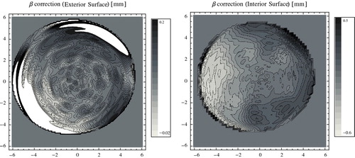
For our data consisting of points representing the corneal surface, we have calculated that , for the exterior and , for the interior corneal surface. Then, calculating (17) with we obtained the -corrections. The integrations for finding the Fourier–Bessel coefficients were done by first interpolating the real data with Lagrange interpolants and then by using the standard numerical quadrature schemes. We kept , for calculations for both surfaces. The corrections are depicted on Figure 1. The absolute fitting error for model and data after applying the correction, that is using , is approximately and  mm for exterior and interior surfaces respectively. This is slightly less than the mean error calculated with and only constant: and  mm. The correction was more successful for interior surface.

Conclusion and discussion

In this paper, we have presented a stable method for solving an inverse problem in a PDE describing the corneal topography. We have developed a regularized solution giving the parameters that are associated with the elasticity and the intra-ocular pressure of the cornea. These in turn have a great impact on the health of the eye. We have acquired a solution by expanding it in an orthogonal basis in . The solution was unstable with respect to the initial noise which made it not usable in applications. We applied the Tikhonov and spectrum truncation regularization methods to overcome these difficulties. The rate of convergence with respect to the noise was also found.

Calculation with the real data gave better results than in the case of constant parameters and . We obtained the profile of the correction which described the cornea in more detail. The mean fitting error is of order of less than one per cent. Moreover, may be a measure of how the intra-ocular pressure deviates from the uniformity. This in turn might prove helpful in diagnosing various corneal conditions. We believe that this model will be useful in understanding and treating different corneal diseases.

Acknowledgments

The authors would like to thank Dr Robert Iskander from Institute of Biomedical Engineering and Instrumentation, Wroclaw University of Technology, Poland and School of Optometry, Queensland University of Technology, Australia for access to the data. This research was supported by the Polish Government funds for science: research project NCN 2012/05/N/ST1/02860.

References

- Trattler, W, Majmudar, P, Luchs, JI, and Swartz, T, 2010. Cornea Handbook. Thorofare: Slack Incorporated; 2010.
- Kasprzak, H, and Iskander, DR, 2006. Approximating ocular surfaces by generalized conic curves, Ophthal. Physiol. Opt. 26 (2006), pp. 602–609.
- Rosales, MA, 2009. M. Juárez-Aubry, E. López-Olazagasti, J. Ibarra, and E. Tepichín, Anterior corneal profile with variable asphericity, Appl. Opt. 48 (2009), pp. 6594–6599.
- Anderson, K, El-Sheikh, A, and Newson, T, 2004. Application of structural analysis to the mechanical behaviour of the cornea, J. R. Soc. Interface 1 (2004), pp. 3–15.
- Ahmed, E, 2010. Finite element modeling of corneal biomechanical behavior, J. Refract. Surg. 26 (2010), pp. 289–300.
- Iskander, DR, Collins, MJ, and Davis, B, 2001. Optimal modeling of corneal surfaces by zernike polynomials, IEEE Trans. Biomed. Eng. 48 (2001), pp. 87–95.
- Schneider, M, Iskander, DR, and Collins, MJ, 2009. Modeling corneal surfaces with rational functions for high-speed videokeratoscopy data compression, IEEE Trans. Biomed. Eng. 56 (2009), pp. 493–499.
- Okrasiński W, P&lslash;ociniczak &Lslash;. Bessel function model for corneal topography; 2011. arXiv:1111.6143v1 [math.AP]..
- Okrasiński W, P&lslash;ociniczak &Lslash;. A nonlinear mathematical model of the corneal shape. Nonlinear Anal-Real. 2012;13:1498–1505..
- Engl, HW, Hanke, M, and Neubauer, A, 2000. Regularization of Inverse Problems. Dordrecht, Boston, London: Springer; 2000.
- Groetsch, CW, 1993. Inverse Problems in the Mathematical Sciences. Braunschweig: Vieweg; 1993.
- Abramowitz, M, and Stegun, IA, 1965. Handbook of Mathematical Functions: with Formulas, Graphs, and Mathematical Tables. New York: Dover; 1965.
- Kirsch, A, 1996. An Introduction to the Mathematical Theory of Inverse Problems. New York: Springer; 1996.