Numerical modelling of slumps under highways located on a mining damage area, based on experimental measurements

Abstract

A system of ground movement measurements under a highway in an Upper Silesia (Poland, Europe) mining damage area has been presented. The objective of the research was to develop a numerical analysis of such slumps occurring under a highway, carried out by a reliable and fast method of converting the results of relevant experimental measurements into ground displacements under the road. For engineering purposes, the results of both monitoring and analysis should be proceeded online, in a fast, sufficiently accurate and reliable way.

Keywords:

• inverse problem
• regularization
• non-linear optimization
• error estimation
• results reliability

Classification:

• 49N45
• 65K10
• 65F22
• 65J20

Introduction

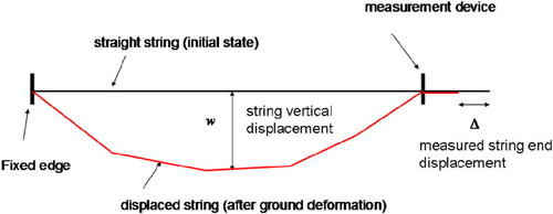
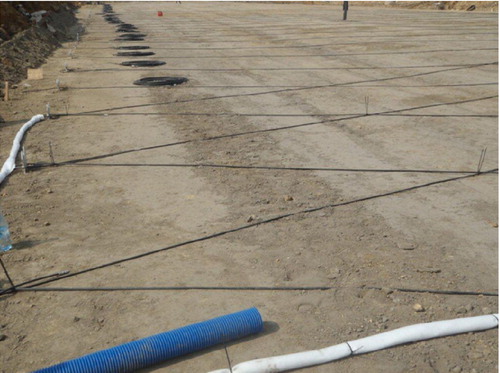
The aim of the paper is to discuss an actual engineering problem of online evaluation of slumps (their location, shape and size) that may develop under the pavement of a highway built on an Upper Silesia mining damage area.[1, 2] The analysis of vertical ground displacements is based on measurements of displacements of flexible strings placed under the monitored highway construction inside protective tubes. The strings form a network consisting of two families of quasi-parallel lines inclined towards each other, and to the road axis at the angle of about 60. Each string is fixed on one road edge, and is free to move on the other one. It is attached to an extensometer measuring the string end displacement resulting from ground subsidence. Additionally, it is assumed that both road edges are immovable. The extent of string displacements depends on the values of vertical ground subsidence. The strings are made of stainless steel covered with a protective coating of polyethylene, and placed inside the protective tubes enabling their free motion. In this way, long life of the effective measurement service of the whole device is secured. Figures 1 and 2 show the location of the measurement elements along the route, and the main principle of operating of the whole measurement system, respectively. Figure 3 presents a photograph of the actual measurement system, taken when it was being fixed along the highway route.

Fig. 1 Location of the measurement elements along the section of the straight route.

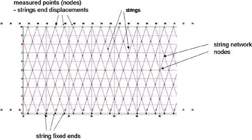
Fig. 2 Diagram of the string displacements and measurement location.

The following assumptions have been made:

•	the strings can move freely inside the protective tubes; they are unstretchable, and do not carry compression,
•	the strings are fixed on one end, and are free to move on the other one; each string end displacement is measured continuously by the extensometer (clip-gage) up to  20 cm,
•	additionally, the vertical displacements of a few selected nodes can also be measured,
•	there are no horizontal constraints between intersecting strings,
•	the vertical displacements of string nodes are restricted by the maximal measured end displacement and therefore cannot be very large compared with the total string length,
•	all strings together form a network covering the whole highway width; the nodes (strings intersections) located on the highway sides do not move, i.e. slumps can only develop under the surface of the pavement.

Since the measurement system has the form of a network of strings, string deflection follows ground displacements – the ground and strings are ‘tied’ at all nodes (points where two strings intersect). Moreover, the ground subsides under the existing highway route; therefore it is not possible to observe the ground deflection itself. The ground remains undeformed as long as the highway is being constructed and the measurement system is established. Ground displacement is expected to happen during highway operation. It is only then that the signals can be emitted from the string deflections. Slumps are created underneath the highway only. The highway and its closest neighboruhood remain unchanged.

The main research objectives of the present paper are to formulate and develop an effective and reliable algorithm providing online information about slumps (location, shape and size) developing under a highway situated on an Upper Silesia mining damage area.

Fig. 3 The actual measurement system, taken when it was being fixed along the highway route (photograph taken by Neostrain Company).

The paper also proposes a modification of the algorithm of the suggested simple procedure to include additional information given in the form of values of the vertical displacements measured at selected points along the road. The points can be located on the centre line of the road.

Problem formulation and modeling

The task can be characterized as a non-linear inverse problem [3]. The experimental measurements of each string end displacement are given while what is searched are the vertical displacements of each node of the strings network (). Additionally, the problem is underdetermined since the number of unknowns () widely exceeds the number of measured displacements (). For instance, in the case of a rectilinear segment of route of the length of 100 m and width of 10 m, using strings spaced every 2 m, the total number of 100 strings is obtained (the number of experimental data ), and 349, 243 nodes of which are located outside the highway edges. The nodal vertical displacements of the nodes constitute a set of unknowns. Consequently, it is not possible to determine the displacements of these nodes on the basis of measurements exclusively, i.e. without either additional data, or complementary information or assumptions. These assumptions may affect the shape of such strings after ground deformation, and consequently, the shape of slumps identified, as well as the behaviour of the string network.

Therefore, the solution algorithm proposed here is based on a reasonable appropriate regularization approach, providing complementary information necessary for the unique solution of the inverse problem in question. Several additional hypotheses about the behaviour of the surface described by the strings network have been proposed and tested. The hypotheses are rather of mathematical nature (however, strings can not be treated as stretchable mechanical cables), and include requirements of either the maximum volume of the slump or its maximum smoothness (minimum of its surface curvature). Obviously, it has to be realized that such assumptions are subjective and affect the final results. In such circumstances, the analyst’s reliability requires to verify whether the various reasonable assumptions considered lead to similar results and are acceptable from the engineering point of view. The analysis carried out by the authors and presented in the paper clearly shows that this is the case.

Adopting any one of these assumptions leads to the mathematical formulation of the problem as a non-linear optimization problem with equality constraints. The objective function proposed here was based either on the slump volume (maximum is searched) as given by the string network or its curvature (minimum is required). The equations describing the strings lengths constitute the constraints. The length of each displaced string must be equal to the sum of the string length before ground deformation and known (measured) end displacement of its end. Thus, non-linearity can occur both in the objective function and the constraints.

These hypotheses were tested on a single string first, adopting an objective function relevant for a 2D analysis (Section Section13). Both the non-linear and linearized forms describing the string length were used. Linearization is justified because vertical displacements of the string network were assumed to be not very large. What was unknown were the vertical displacements of nodes. Additional assumptions introduced lead to the non-linear constrained optimization problem [4] solved first by means of the iterative Newton–Raphson method [5]. As an initial solution, nodes locations prescribed by the relevant parabolic curves of each string were applied. After a variety of calculations for networks with a regular and irregular distribution of nodes were performed, it was found, as expected, that all variants of additional assumptions applied actually yield very similar final results. Moreover, the solution modelled by means of a parabolic curve is relevant to the maximum area rule with the linearized constraint conditions. Therefore, a new formulation of the task for a single string was considered. Each string was assumed to be of a parabolic shape. Consequently, as the location of the string ends is known, the only unknown parameter in the string form is the vertical displacement value of its middle point. The displacements of all remaining nodes will be computed according to the parabola shape. The unknown value can be obtained using either the linearized explicit formula, or by means of a simple iterative procedure (Newton’s tangent method, [5]) for one non-linear equation only (the exact value). Both results have proved to be very close to each other, and the first one presents an excellent starting value for the iterative approach.

Such formulated task of analysis of a single string vertical displacements was extended to the whole network system (Section Section14) in order to develop a simplified but reliable solution algorithm, precise sufficiently to provide effective engineering results. Once the network has been generated, the algorithm for a single string (described above) runs one by one for each string. As a result, two displacement values are obtained for each node found for each pair of two intersecting strings. In this way information overload is dealt with. Two complete independent solutions can then be defined (‘left’ for one full set of quasi-parallel strings and ‘right’ for the other one) for the entire network. Next, these two solutions are averaged. Determination of such averaged solution ends the simplified procedure. It is fast (online speed), simple and very accurate. The only error introduced into the measured displacements results from the averaging procedure. A variety of tests done indicated the effectiveness of this procedure for both the straight (simulated) and curved (real) roads. Selected results are presented below.

Moreover, a more rigorous approach was discussed and tested for comparison. The whole string network was analysed simultaneously (Section Section15). Eventually, the analysis of results reliability was carried out (Section Section16) to justify the application of the simplified solution approach. It is worth noticing that the initially underdetermined constrained optimization problem was finally converted into an overdetermined one.

Analysis of a single string

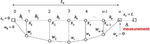
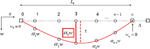
An example of a string with nodes (numbered ) arbitrarily distributed is presented in Figure 4. The following are given: coordinates of all nodes , displacements of the string ends (boundary conditions ), string length(1) before the ground deformation as well as the measured string end displacement . What is searched are nodes displacements .

Fig. 4 Analysis of a single string.

The adopted constraints result from the string length equation(2) in which(3) denotes the string length after ground deformation. The regularization approach is applied now. The following hypotheses were adopted from the 3D space mentioned before, and proposed in order to evaluate the displacements of nodes for a single string:

•	concept of the maximal surface area defined (Figure 4) by a figure bounded by the initial position of the string (undeformed) and the displaced one;
•	concept of the minimal curvature (maximal smoothness) of the curve defined by the nodal points after the string displacement.

In both these cases, the horizontal displacements are neglected.

Concept of the maximal surface area

The total surface area above the displaced string can be written as:(4) A corresponding non-linear optimization problem can be formulated as follows: find the stationary point of the Lagrange function(5) subjected to the constraints (2) and (3). Hence, the stationary conditions are(6) Linearized version of can be formulated as well. It is based on the equation(7) which holds for . For instance, for real data , , which is a relative small number. Such ratio comes from the analysis of the string of typical length as well as from the maximal deflection that can be measured by the system (20 cm). However, in further iterative approach, the square root of is evaluated in the exact numerical manner.

Minimal string curvature (maximal smoothness) concept

Simplified curvature of a displaced string at the specified node(8) can be evaluated by means of a relevant difference formula for the second derivative(9) taking advantage of the arbitrarily distributed nodes at the string. The total curvature of the displaced string is a sum of all nodal curvatures(10) In such case, the Lagrange function can be written in the following form(11) Its linearized version can also be formulated. The stationary conditions are the same as in the previous case (6).

Numerical results and conclusions

A string of the length and measured displacement (which constitutes the maximal displacement value that can be measured by means of the applied measurement system) were analysed. Numerical tests concerned both strings with regular and irregular distribution of nodes. In each case, the initial values of nodal displacements (for non-linear case without any additional linearization) were based on the parabola shape. Next, the Newton-Raphson method was applied in order to solve numerically the set of Equations (6) with the required accuracy of of the relative solution error. The summary of results (I – maximal surface area with the linear string length, II – maximal surface area with the non-linear string length, III – minimal curvature with the linear string length and IV – minimal curvature with the non-linear string length) is presented in Figure 5 and Table 1 for the mesh with seven regularly spaced nodes as well as in Figure 6 and Table 2 for seven nodes distributed irregularly.

Fig. 5 Results summary for regularly distributed nodes.

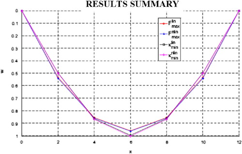
Table 1 Results summary for regularly distributed nodes.

Case
I(lin, max )	0.5345	0.8552	0.9621	7.4833	0.0286
II(nlin, max )	0.5421	0.8599	0.9647	7.5373	0.0294
III(lin, min )	0.4988	0.8640	0.9976	7.4462	0.0268
IV(nlin, min )	0.5014	0.8693	1.0043	7.4915	0.0271

Fig. 6 Results summary for irregularly distributed nodes.

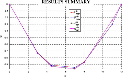
Table 2 Results summary for regularly distributed nodes.

Case
I(lin, max )	0.72747	0.90934	0.94302	0.86219	0.29638	7.4299	0.029038
II(nlin, max )	0.73378	0.19329	0.94643	0.86707	0.30331	7.4746	0.030050
III(lin, min )	0.72394	0.92650	0.96185	0.86616	0.24003	7.3775	0.026098
IV(nlin, min )	0.72782	0.93204	0.96814	0.87181	0.24148	7.4225	0.026420

All variants, i.e. non-linear and linearized versions as well as both criteria (maximal volume and minimal curvature), provide almost the same results, with precision sufficient for engineering purposes. Moreover, the results obtained for the linearized maximal surface area concept are the same as the initial solution based on the parabola shape. Therefore, the use of only the simplest formulation, i.e. the linearized maximal volume concept that is equivalent to nodes location on parabola, is fully justified. Although the above results were presented for seven nodes on the string, the same similarity of results is observed when applying configurations with a smaller number (two to six) of nodes placed on the vertically displaced part of the string.

Final algorithm applied for a single string and results of numerical analysis

Following the conclusions drawn above, some simplifying assumptions are introduced: all displaced nodes(12) are situated on the same parabola, described by the string ends (zero displacement values) and its middle point, assuming its value to equal one. Coefficients can be calculated using the implicit quadratic relation(13)

Fig. 7 Distribution of the string displacements for adopted parabolic shape.

Finally, all nodal displacements are determined by the string end displacement and controlled by the maximal value , see Figure 7.

Therefore, there is only one unknown string displacement instead of unknown nodal displacements. It can be evaluated either using the linearized formula(14) or by means of a numerical analysis of non-linear Equation (2) taking into account the unchanged string length constraint(15) and application of the Newton tangent method with the initial solution defined by (14)(16) in which(17) The brake-off condition of the iterative process (16) is based on an appropriate level of the relative solution error, describing the procedure convergence, as well as the residual error, controlling the solution quality. Below, some examples of results for the regular mesh with seven nodes, regularly distributed, with nodal values placed on the parabola are presented. The coefficients (13) are , hence the result of the linearized solution (14) is 0.9621. Thus, all nodal displacements are . Next, the non-linear solution can be obtained by means of the Newton iteration process (16). Eventually, the improved values of all nodal displacements are . The same similarity in results can be observed when the irregular mesh is taken into account.

Simplified analysis of the string network

In the previous section, the concept of evaluation of the vertical nodal displacements of a single string was presented. Before analysing the entire string network, information about the network topology has to be prepared, i.e. the positions and mutual relations between strings and nodes. The algorithm presented in this section provides distinction between the ‘left’ and ‘right’ strings. This division results from the specificity of the measurement system in which two strings converge or intersect in each node. Those strings can be inclined ‘positively’ (at an acute angle) or ‘negatively’ (at an obtuse angle) with respect to the edge lines of the route. The idea of a simplified network analysis lies in the fact that for each string the vertical displacement can be determined individually on the basis of the algorithm presented in the previous section. Due to the adoption of the parabolic shape of the deformed string the problem of information overload appears. Two independent configurations of solutions will be provided, namely the ‘left’ and ‘right’ solutions, which will be averaged. This averaging procedure introduces certain errors and, therefore, the final configuration may not satisfy the exact equations of the displaced strings lengths (2) and (3). However, it will be shown that such averaged solution constitutes, from an engineering point of view, very good approximation to the exact solution, obtained simultaneously for the entire network. Furthermore, it should be emphasized that obtaining such a solution is a very fast, almost online process. This procedure of evaluation of the entire string network displacements, based on the displacement of each string separately, and followed by the averaging procedure, will be called ‘simplified’ and its result – the ‘simplified’ solution. The simplified solution may also be an effective initial point for numerical analysis of the exact non-linear system of equations simultaneously built on the level of the whole network.

Problem formulation and solution approach

The analysis is based on experimentally measured displacements of each string end. The maximal displacements of each string are searched. Due to the parabola shape assumed for strings, it is a case of an overdetermined problem type, in which the number of known values exceeds the number of unknown values of . Solution approach of the simplified procedure consists of the following steps applied subsequently to each single string:

•	Find the coefficients using the formula (13), corresponding to the parabolic shape of each deformed string.
•	Find the maximal displacement of each string using its measured displacement and explicit formula (14) for the linearized case or the iteration process (16) for the non-linear one (15).
•	Evaluate all nodal values of string displacements.
•	Next, select from the whole network two families of quasi-parallel strings (‘left’ and ‘right’). Each of these families provides a complete solution for nodal displacements in the entire network.

The final simplified solution can be found by means of the averaging procedure(18) while the solution error bounds can be estimated as follows:(19) In another error estimation technique of residual nature, the equations of string lengths (2) can be used in which the displacement can be evaluated either on the basis of the exact measurements () or on the basis of the simplified solution. The comparison of these two length quantities for each string(20) provides information about the error value in satisfying the optimization constraints.

Numerical examples

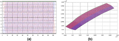
Two types of highway routes were examined: Highway #1, a simulated rectilinear route, 100 m long, 10 m wide with strings located every 2 m, which gives the total number of 100 strings and 349 nodes (Figure 8(a)). The other Highway #2, a real curving route, of length of 402 m, width of 77 m and strings located every 2–2.5 m, which gives the total number of 348 strings and 1884 nodes (Figure 8(b)).

Fig. 8 Straight route - Highway #1    Curved route – Highway #2.

Further analysis requires knowledge of (measured) string displacements . Since the results of actual measurements were not available when the present study was being conducted, measurements had to be simulated for testing purposes. Several various configurations of ground displacements under the monitored highways were simulated by means of mathematical criteria only, applied to determine the slump shape. Non-polynomial functions were adopted because the simplified procedure is based on the parabolic (polynomial) shape of the deflected string. The trigonometric function was applied for Highway #1 while a spherical surface was applied for Highway #2. 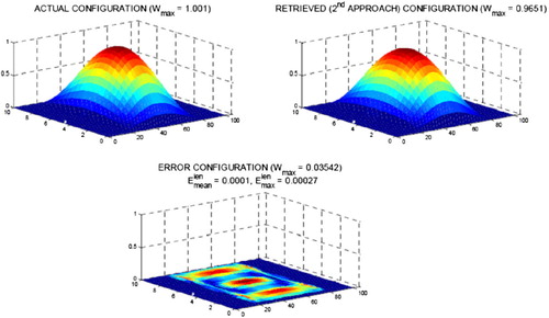The string end displacements were calculated (simulated measurements) corresponding to the slump form assumed and resulting nodal displacements of the entire network. Several detailed results, obtained by means of the Matlab package,[6] are presented below for configuration of Highway #1 with one large slump under the pathway. Figure 9 shows ‘left’ solution (top left), ‘right’ solution (top right), difference between them (bottom left) and simplified solution – the average of ‘left’ and ‘right’ solutions (bottom right). The maximal values of displacements are provided in the graph labels. Figure 10 shows the final results: the exact (actual) solution used for simulation of measurements (top left), simplified (retrieved) solution (top right) as well as solution error – difference between these solutions (bottom left). The maximal error calculated on the basis of the string length Equation (20) is 0.0027%.

Fig. 9 Detailed results for Highway #1 – displacement configuration with one slump.

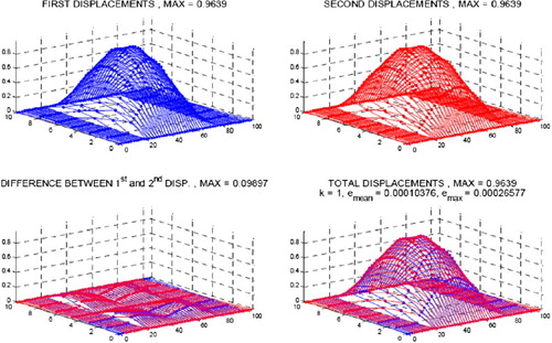
Fig. 10 Final results for Highway #1 – displacement configuration with one slump.

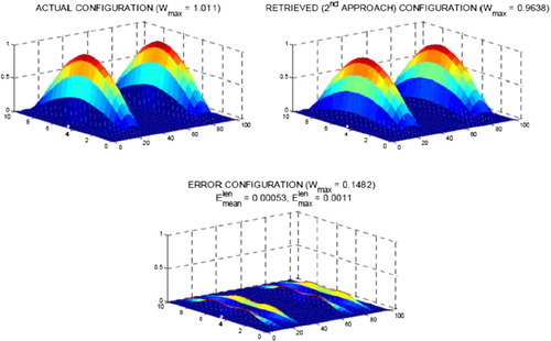
The same set of results was prepared for many other simulated configurations. However, due to the format of the present paper, only selected results will be presented herein. The final results for configuration with two slumps are shown in Figure 11. The maximal error calculated on the basis of the string length equations is 0.0011%.

Fig. 11 Final results for Highway #1 – displacement configuration with two slumps.

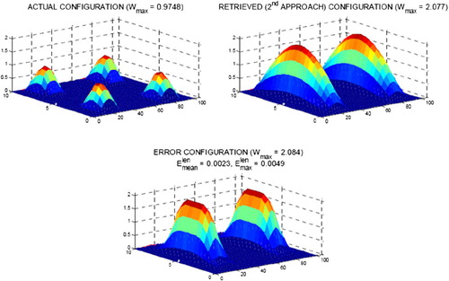
The simplified procedure cannot reconstruct true shapes of all the types of slumps. For instance, if two or more independent slumps are formed along the width of the road, it is not possible to distinguish one from another one clearly using this procedure (Figure 12). However, it has to be stressed that this results from an insufficient number and type of initial experimental data.

Fig. 12 Final results for Highway #1 – displacement configuration with four slumps.

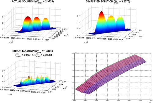
Figures 13 and 14 give the final results (exact solution – top left, simplified solution – top right, solution error – bottom left, route and string network – bottom right) for Highway #2, for configuration with one slump – Figure 13 – and three slumps – Figure 14. The maximal errors calculated on the basis of the string length equations are 0.0060% for one slump and 0.0068% for three slumps.

Fig. 13 Final results for Highway #2 – displacement configuration with one slump.

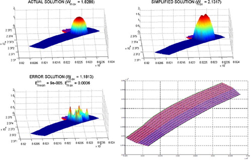
Fig. 14 Final results for Highway #2 – displacement configuration with three slumps.

Additional measurement data

The simplified procedure can be effectively modified in order to adopt additional geodetic measurement data [2]. These data can be divided into two groups:

•	Vertical displacements of selected points along the route, whose position is given. In the simplest case, these points are located on the centre line of the route, through a distance of 50 m. Ground displacement monitoring at these points is carried out continuously. Therefore, the solution algorithm can be updated with this type of information any time.
•	Vertical displacements of selected points along the straight sections spaced at 50 m, measured through the edges and the centre line of the road. The measurement at those points is done only occasionally.

Several possible extensions of the simplified procedure can be proposed in order to investigate both types of additional data. The most reliable one seems to be simultaneous application of both measured data (string displacement and displacement of its central point ) by means of the following procedure. In the first stage displacements of all string nodes are calculated, on the basis of the measured displacement of the string middle point . Next, the corresponding string displacement is calculated, which will be, in general, different from the measured one . Eventually, the averaged measurement data are evaluated(21) Once again the simplified solution is found for such modified data. The final result, i.e. nodal string displacement, will be based on both types of information (displacements of the string and displacement of its middle point).

Conclusions

To summarize briefly the simplified procedure, let us highlight several advantages of this approach: simplicity, computational speed (online results), easy implementation, high-quality results and excellent initial solution for Newton–Raphson procedure, if needed. The proposed approach has virtually no disadvantages. The only error in the final solution comes from the averaging procedure of two solutions for each string in the network, but it was found to be negligible.

Simultaneous analysis of the entire string network – a rigorous solution approach

The application of the simplified procedure has shown that the solution obtained in this way may be a very good approximation of the exact solution with respect to the given measured string ends displacements. Moreover, the simplified solution is obtained relatively very fast and without difficulties. However, there is also a possibility of obtaining exact solutions satisfying (with a specified accuracy) simultaneously all displacement equations for all strings at once. Such an approach yields rigorous analysis of the entire string network and leads (using additional assumptions) to a large non-linear system of equations for the unknown vertical displacements of all nodes.

Exact problem formulation

Regularization approach has been limited herein to the maximal volume concept only. Volume will be treated as the total surface area between all deformed and undeformed strings containing unknown nodal displacements(22) Each -th string contains nodes numbered . Length equations for each string constitute corresponding constraints(23) Lagrange function(24) depends on the unknown nodal displacements and Lagrange multipliers . Stationary conditions are(25) The Newton–Raphson solution procedure was applied. The simplified solution described in the previous section was used as the starting point in the iteration procedure. Relevant brake-off criteria, controlling both the solution and residual errors, were adopted.

Numerical examples

A numerical analysis of selected configurations of Highway #1 was carried out by means of a more rigorous, complex approach described in the previous subsection. The summary of the iteration procedure applied for the set of non-linear Equations (25) is presented in Figure 15. The figure shows the convergence paths for both solution and residuum, for vertical displacements (top graph) and for Lagrange multipliers (bottom graph), separately. The final results for the configuration with two slumps placed along the straight route are presented (Figure 16):

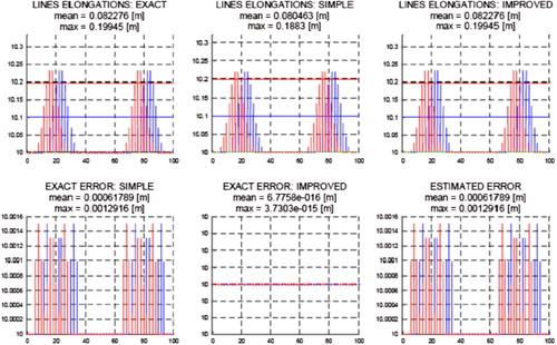
•	In the first row, the previous results of the simplified method are shown: comparison of the exact solution with the simplified one, and its error when compared with the first one. The maximal relative solution error is , whereas the maximal error calculated on the basis of the string lengths equations is ,
•	In the second row results of the rigorous method are given: comparison of the exact solution with the rigorous solution, and its error with respect to the exact solution. The maximal relative solution error is , whereas the maximal error calculated on the basis of the string lengths equations is .

Figure 17 shows a comparison of the string end displacements , along the top edge of the road. In the first row, (in the same scale) from left to right, initial string end displacements (simulated measurements ), string end displacements retrieved after obtaining the simplified solution () and string end displacements retrieved after obtaining the rigorous solution are given (). The second row presents (in the same scale) their differences (exact and estimated errors of the string end displacements), from left to right: exact error based on the simplified solution , exact error based on the rigorous solution and estimation of the first error . The string end displacements error based on the rigorous solution equals zero, the estimation mentioned above is exact. The mean and maximal values of these non-relative errors are shown within the labels of each component graph.

Fig. 15 Summary of the iteration procedure – Highway #1 – configuration with two slumps.

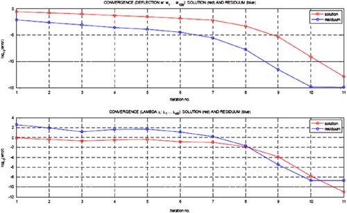
Fig. 16 Exact solution (upper left and lower left graph), the simplified solution (upper middle graph), the rigorous solution (lower middle graph), the simplified solution error (upper right graph) and a rigorous solution error (bottom right graph) – Highway #1 – configuration with two slumps.

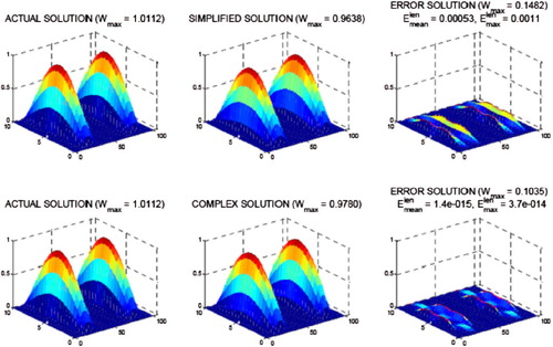
Fig. 17 Comparison of the string end displacements for three solutions: exact, simplified and rigorous ones, as well as appropriate errors of the numerical solutions.

As can be noticed, there is no substantial difference between the solution obtained by means of the simplified and rigorous methods, when the maximal displacement, shape or volume are taken into account. However, the length balance Equations (2)–(4) are satisfied in the most exact way in the case of the rigorous approach. Therefore, it is one and the only visible advantage of such approach. Moreover, this approach is much more computationally demanding. On the other hand, the simplified procedure may be successfully applied to estimate the extent of ground displacements. It is fast, simple and accurate. The most rigorous, most accurate procedure, described in this section yields a nearly identical solution, although it takes a much longer time. In addition, it should also be noted that the rigorous procedure may be unstable and divergent. The authors of the present study were confronted with these cases when calculating the displacement of some selected configurations for Highway #2. However, if the process is convergent, then the complex procedure can be applied to validate the simplified solution if needed.

Reliability analysis

Taking into account the actual target, i.e. engineering application of the method developed and presented in the paper, the reliability of the analysis proposed should be examined carefully. High reliability of the proposed simplified solution approach was found and demonstrated herein. It can be confirmed by:

•	A variety of tests done for a single string including comparison of: • two criteria of regularization, • regular and irregular networks, • non-linear and linearized algorithms, • only vertical displacements of nodes vs. vertical and horizontal ones. Each time the results obtained were very close to each other.
•	Availability of two independent ‘left’ and ‘right’ solutions for the whole mesh. This fact allowed both averaging the results and evaluation of their error bounds. These solutions were also found to be close to each other.
•	Possibility of strict evaluation of the difference between displacements of the strings end measured and calculated for the slump form determined by the averaged solution.
•	Direct comparison of the simplified averaged solution with the results of tests where rigorous (exact) numerical solution was found (Highway #1). Both solutions were very close to each other.

Final remarks

A real engineering problem of online evaluation of slumps that may develop under the pavement of a highway situated on an Upper Silesia mining damage area [1, 2] has been investigated. The results have been obtained by frequently repeated measurements of displacements of strings ends, fixed under the pavement (inside the protective tubes). The displacements were indication of ground subsidence. In general, reconstruction of each slump cannot be done successfully when based on the experimental measurements of ends strings exclusively, because such problem is underdetermined. The number of unknowns clearly prevails over the number of available experimental data. The problem can be solved when aided by a regularization approach [3]. Two criteria for such approach were proposed and tested, namely the maximal volume of a slump in question or minimal curvature (or maximal slump smoothness) of its surface. From the engineering point of view both ways provided very close results. The problem is then formulated as non-linear optimization of the Lagrange type function [4]. A complete rigorous numerical solution of such a problem yields the analysis of simultaneous non-linear algebraic equations, solved by means of the Newton–Raphson procedure [5]. Such a solution can be reached with high a-priori required precision. The solution procedure, when convergent, is relatively fast, but not sufficient for engineering purposes. Therefore, a simplified solution approach has been developed. First, all strings, one by one, are analysed separately. The analysis of each one requires a solution of one non-linear algebraic equation with one unknown only because the string displacements were assumed as described by the parabola shape. Following this assumption, the number of available experimental data becomes twice bigger than the number of unknowns. The results of analysis of each string are next collected in two files, denoted as ‘left’ and ‘right’ global solutions (provided by each of two groups of quasi-parallel strings). Their average presents the required final solution while their difference provides an error evaluation. The simplified solution satisfies all the requirements imposed on the engineering approach. It is convergent, simple and precise. It is very fast (practically online speed), and is easy in implementation. It is reliable and its error bounds are easily evaluated. The results obtained from the simplified procedure are very close to those found by means of the rigorous numerical approach. All calculation results providing information about slumps development are well visualized,[6] and can be observed any time online. It should be remembered, however, that both the simplified and rigorous procedures suffer from insufficient number of the initial data and, therefore, may not be able to fully reconstruct the true slumps shape.

However, all the formulations of the problems and their solutions discussed above have been done so far based on too restrictive and rather non-realistic assumption: none of the nodes on the highway sides move (i.e. slumps may only develop under the surface of the pavement). Moreover, there could also occur horizontal displacements of the highway edges due to thermal or water infiltration processes. In the future analysis such restrictions can be removed by

•	monitoring highway sides motion by appropriate measurements, e.g. based on the GPS technique,
•	decomposition of the total ground displacements into motion of highway surface (new part) and formation of underground slumps (old part).

Other recommended future plans, important from the engineering point of view, include

•	possibility of dealing with incomplete or erroneous data (e.g. due to wrong reading, broken strings, ...),
•	optimal choice of the number and location of strings, especially in curved sections of the highway.

References

- Bednarski L. Project of monitoring of soil vertical displacements and deformation of geo-network – designed by the Inora and Neostrain Companies: Cracow; 2010..
- Collective work, Surface protection against effects of mining solid deposits (in Polish), Wydawnictwo Ślask, Katowice, Poland (1980)..
- Dulikravich GS, Tanaka M. Inverse problems in engineering mechanics III. 1st ed. Amsterdam: Elsevier Science; 2001..
- Pierre, D, 1969. Optimization theory with applications. New York, USA: John Wiley and Sons, Inc.; 1969.
- Press WH, Teukolsky SA, Vetterling WT, Flannery BP. Numerical recipes, the art of parallel scientific computing. New York: Cambridge University Press; 1999.
- Dulikravich G.S., Tanaka.M, Inverse Problems in Engineering Mechanics III, 1st Edition, Elsevier Science (2001)..