Inverse source problem in a one-dimensional evolution linear transport equation with spatially varying coefficients: application to surface water pollution

Abstract

This paper deals with the identification of a time-dependent point source occurring in the right-hand side of a one-dimensional evolution linear advection–dispersion–reaction equation. The originality of this study consists in considering the general case of transport equations with spatially varying dispersion, velocity and reaction coefficients which enables to extend the applicability of the obtained results to various areas of science and engineering. We derive a main condition on the involved spatially varying coefficients that yields identifiability of the sought source, provided its time-dependent intensity function vanishes before reaching the final monitoring time, from recording the generated state at two observation points framing the source region. Then, we establish an identification method that uses those records to determine the elements defining the sought source. Some numerical experiments on a variant of the surface water pollution model are presented.

Keywords:

• inverse source problem
• optimization
• partial differential equations
• advection–dispersion–reaction equations
• environmental monitoring: surface water pollution

Introduction

Inverse problems play a key role in providing estimations of unknown and sometimes even inaccessible elements involved in the associated mathematical model using some observations of its response. In real world problems, having an accurate estimation of the missing elements in the mathematical model usually leads to a better understanding of the occurring phenomena and thus, to take appropriate actions in order to prevent undesirable situations. During the last few decades, we have seen inverse problems to be employed in numerous areas of science and engineering: in medicine, the inverse problem of electrocardiography, for example, is used to restore the heart activity from a given set of body surface potentials [1]. In seismology, inverse source problems are used to determine the hypocenter of an earthquake [2] as well as to study the dynamic problem of seismology which is one of the most topical problems of geophysical [3].

A motivation for our present study concerning inverse source problems in transport equations is a typical problem associated with environmental monitoring which can be described as follows: certain areas like water, groundwater or atmosphere can be monitored by some sensors destinated to evaluate the level of pollution in the site. When the incoming signals reveal an unusual rise in pollution concentrations, the top priority action becomes the identification of the contamination source as quickly as possible in order to prevent worse consequences. A concrete example of this situation consists of the identification of pollution sources in surface water: in a river, for example, the oxidation of organic matter introduced by city sewages, industrial wastes, etc. usually drops to too low the level of dissolved oxygen in the water. Problems with low concentrations of are essentially an unbalanced ecosystem with fish mortality, odours and other nuisances, see [4] for more details. Therefore, as soon as the sensors begin to inform about a lack of , the identification of pollution sources becomes a priority in order to preserve the diversity of the aquatic life and prevent many species from perishing. That also enables an alert to downstream drinking water stations about the presence of accidental pollution. The identification of sought pollution sources in a river could be done by monitoring the (BOD) concentration which represents the amount of dissolved oxygen consumed by the micro-organisms living in the river to decompose the introduced organic substances [5, 6]. Thus, the more organic material there is, the higher the concentration.

In this paper, we assume monitoring a portion of a river assimilated to a segment of a line and are interested in the identification of an unknown pollution source responsible of the higher concentrations recorded by some sensors already placed in this portion. The paper is organized as follows: Section 2 is devoted to stating the problem, assumptions and proving some technical results for later use. In Section 3, we prove under some reasonable assumptions the identifiability of the sought source from recording the generated state at two observation points framing the source region. Section 4 is reserved to establish an identification method that uses those records to determine the elements defining the sought source. Some numerical experiments on a variant of the surface water pollution model are presented in Section 5.

Mathematical modelling and problem statement

We suppose monitoring a portion of a river represented by the segment during a time . The concentration, denoted here by , in this portion is governed by the following one-dimensional parabolic partial differential equation, see [7, 8]:(1) where represents the pollution source, is the flow velocity and , are respectively the dispersion and reaction coefficients. Here, is a positive real number, is a function of -class on whereas is a twice piecewise continuously differentiable function on such that for all . The Equation (1) is equivalent to(2) with and . Then, multiplying (2) by the weight function defined as follows:(3) implies that the concentration satisfies(4) where is the following parabolic differential operator:(5) with . As far as initial and boundary conditions are concerned, one could consider without loss of generality no pollution occurring at the initial monitoring time and thus, a null initial BOD concentration. In addition, as the main transport is naturally oriented downstream, it seems to be reasonable the use of an homogeneous Dirichlet upstream boundary condition. However, at least two options are available for the downstream boundary condition: a null gradient concentration or simply a null concentration. This last option is usually employed when the downstream boundary is assumed to be far away enough from the source position. In this paper, we use the following homogeneous initial and boundary conditions:(6) Notice that due to the linearity of the operator introduced in (5) and in view of the superposition principle, the use of a non-zero initial condition and/or inhomogeneous boundary conditions do not affect the results established in this paper.

Furthermore, it is well known that under reasonable assumptions on the regularity of the source , the problem (4)–(7) admits a unique solution smooth enough to use its value at any point of , see [9]. Therefore, given two observation points and such that , we can define the following observation operator:(7) This is the so-called direct problem.

The inverse problem with which we are concerned here is: assuming available the records of the concentration at the two observation points and , find the source such that(8) The main difficulty in such kind of inverse problem is that in general there is no identifiability of the source in its abstract form, see [10]. In the literature, to overcome this difficulty authors generally assume available some a priori information on the source : for example, time-independent sources are treated by Cannon in [11] using spectral theory, then by Engl et al. in [12] using the approximated controllability of the heat equation. The results of this last paper are generalized by Yamamoto in [13, 14] to sources of the form where and the time-dependent function is assumed to be known and satisfying the condition . Furthermore, Hettlich and Rundell addressed in [15] the inverse source problem for the heat equation with sources of the form where is a subset of a disc. They proved the identifiability of from recording the flux at two different points of the boundary. El Badia and sHamdi studied in [10, 16] for a one-dimensional evolution linear transport equation with constant diffusion, velocity and reaction coefficients the identification of a time–dependent point source where the source position and the time–dependent intensity function are both unknown. They proved the identifiability of from recording the state and its flux at two observation points framing the source region. Those results for the case of linear transport equations with constant coefficients have been recently improved by Hamdi in [17, 18] to requiring only the record of the state at the two observation points.

The originality of the present study with respect to [17, 18] consists in considering the underlined inverse source problem in the general case of linear evolution transport equations with spatially varying diffusion, velocity and reaction coefficients. That increases the degree of difficulty and makes the results established in [17, 18] with constant coefficients do not apply at least for the two following reasons: 1. In [17, 18], the essential ingredient of localizing quasi-explicitly the position of the sought source is the use of the impulse response to the operator that is the adjoint of the spatial part of the operator introduced in the left-hand side of (2) with constant , and coefficients. Then, this impulse response is explicitly determined as the solution to a second order linear differential equation with constant coefficients. In the present study, that does not apply with arbitrary spatially varying , and coefficients 2. In [17, 18], by employing a change of variable, the operator in the left-hand side of (2) with constant , and coefficients is transformed into a symmetric operator (the heat equation). And thus, to recover the source intensity function, one solves a deconvolution problem where the associated state is expressed in the complete orthogonal family made by the classic Laplacian eigenfunctions. In this paper, the non-symmetry in the spatial part of the operator introduced in the left-hand side of (2) requires the determination of an adequate weight function that transforms the problem of finding a complete orthogonal family into solving a generalized Sturm–Liouville eigenvalue problem. Then, conditions on the spatially varying coefficients need to be found in order to deal with a regular Sturm–Liouville problem.

According to the usual mathematical modelling of a time–dependent point source, we use in this paper a source that takes the form(9) where denotes the source position and designates its time–dependent intensity function. Moreover, employing a source of the form (10) implies that the problem (4)–(7) admits a unique solution that belongs to:Furthermore, assuming the time–dependent intensity function vanishes before reaching the final control time which means(10) implies that for all . Then, we introduce the following Sturm–Liouville problem:(11) where and are the two functions given in (3). Since , , and are continuous on while and on , the system (12) is a regular Sturm–Liouville problem.[19] Therefore, the eigenvalues for are real, simple and can be ordered such that with . In addition, the normalized eigenfunctions associated to the eigenvalues for form a complete orthonormal family of (12) and for each , the series converges to in .

Remark 1.1In [20], the author proved that if the function belongs to and satisfies the same boundary conditions i.e. , then the expansion converges absolutely and uniformly to in .

Besides, we remind the concept of a strategic point as introduced by El Jai and Pritchard in [21] and employed by the authors in [10, 16].

Definition 1.2 A point of is called strategic with respect to a complete orthogonal family of continuous functions if for all .

Let and be two real numbers such that . For reasons to be explained later, we introduce the following two functions and which are the impulse response to the operator that is the adjoint of the spatial part of the operator introduced in (5):(13) Then, we prove that under a reasonable condition on the spatially varying coefficients , and , the function introduced in (14) does not admit any root in the interval :

Lemma 1.3 Provided the coefficients , and satisfy the following condition:(14) the function introduced in (14) is such that for all .

Proof   As the function introduced in (3) is strictly positive on , satisfies:(15) Then, using , the Equation (16) is equivalent to(16) where the function is defined, in view of (3), as follows:(17) Since for all in , then in view of the last equality in (18), the assertion (15) yields for all in . Therefore, as proved in [22], all solutions to (17) are non-oscillating solutions in . That implies has at most one root in . Furthermore, as and have the same roots and , we conclude that for all in .

That leads to establish the following theorem:

Theorem 1.4 If Lemma 2.3 applies, then the function defined as follows:(18) is continuous and strictly monotonic.

Proof   In view of (14) and using Lemma 2.3, the function introduced in (19) is smooth enough on and we have(19) Besides, according to (14) we find(20) which implies that(21) Then, in view of (20) and (22), the function satisfies in the following second order differential equation:(22) which leads to where is a real constant. Therefore, as according to (3) we have for all in , it follows that the function has a fixed sign on . That implies is a strictly monotonic function on .

To establish the identifiability theorem, we also need to prove the following lemma:

Lemma 1.5 Let be a strategic point with respect to the family as introduced in definition 2.2. If the solution to the following system:(23) satisfies for all in , then we have in .

Proof   Using the complete orthonormal family , we express the solution to the system () at the strategic point as follows:(24) Then, since belongs to and in view of Remark 2.1, it follows from the uniform convergence in of the expansion of in the complete family that in particular we have(25) Furthermore, (26) implies that the series occurring in the right-hand side of () converges uniformly in and represents a real analytic function with respect to the variable . That gives a sense to for . Therefore, as we have(26) it follows by analytic continuation that(27) Then, by rewriting () as follows:and setting the limit when tends to , we find . Hence, by repeating the same principle for all , we obtain(28) Since is a strategic point with respect to the family , we conclude in view of () that for all which implies in .

Identifiability

Provided the main condition (15) holds true, we prove in this section that assuming the time–dependent intensity function satisfies (11), the elements defining the source introduced in (10) are uniquely determined from recording the state solution to (4)–(7) at two observation points and framing the source region. Note that in the case of constant coefficients , and the main condition (15) is equivalent to which is always fulfilled. Therefore, the following theorem can be seen as a generalization of the identifiability result obtained in [18] for the case of equations with constant coefficients:

Theorem 1.6Let where is a positive function of that satisfies (11) and is such that , for . Provided the main condition (15) holds true and at least one of the two observation points , is strategic with respect to the complete orthonormal family , we have(29) Proof   Let be the solution to the system (4)–(7) with the time–dependent point source , for . Then, the variable satisfies(30) Since and satisfy (11), we obtain from multiplying the first equation in (31) by the function solution to the first system in (14) and integrating by parts over using Green’s formula where , then by the function solution to the second system in (14) and integrating by parts over using Green’s formula that(31) where for and the coefficients , are such that(32) Furthermore, as in view of (14) we have , and according to (9), implies that(33) Then, the coefficients and introduced in (33) are reduced to(34) Besides, as (11) holds, then for the variable satisfies in a system similar to the problem (31) where the right-hand side of the first equation vanishes and the initial condition is . Then, assuming the observation point to be strategic and using, in view of (34), in we obtain by applying Lemma 2.5 with that in . Therefore, according to (35) that leads to find . In addition, since the main condition (15) holds, we have according to Lemma 2.3 that and . Thus, using (32), we find(35) where is the function introduced in (19). From (36) and using Theorem 2.4, we obtain . Now, by setting we have(36) Then, using the complete orthonormal family to compute the solution of (37) and the Titchmarsh’s theorem on convolution of functions [23], we prove by employing similar techniques to those used in [10] that the assumptions is a strategic point and for imply that almost everywhere in .

Identification

In this section, we focus on establishing an identification method that uses the records (9) to determine the elements defining the source introduced in (10). To this end, we proceed in two steps: a first step enables to localize the source position and compute the mean value of the loaded intensity function . Then, a second step uses the determined source position and transforms the recovery of into solving a deconvolution problem.

Step1: Localization of the source position

Proposition 1.7 Let be a time–dependent point source as introduced in (10) where satisfies (11) and let . Provided the coefficients , and satisfy the main condition (15), the source position and are subject to:(37) where , are the two functions introduced in (14), (19) and , are such that(38) Proof   Let be the solution to (4)–(7) with the time–dependent point source introduced in (10). Since (11) holds, we obtain from multiplying the equation (4) by the function solution to the first system introduced in (14) and integrating by parts over using Green’s formula where , then by the function solution to the second system in (14) and integrating by parts over using Green’s formula that(39) where and the coefficients , are given by(40) Therefore, using the boundary conditions on and , in (41), we find the coefficients and introduced in (39). Furthermore, since the main condition (15) holds we have according to Lemma 2.3 that . And thus, from (40) we obtain the result announced in (38).

Remark 1.8 Note that as is subject to only knowledge of and for , the computation of the source position and from (38) is not so far possible since the coefficients and derived in (39) still involve the unknown data .

To determine the two integrals in (39) involving the unknown data , we prove the following proposition:

Proposition 1.9 Assuming (11) holds, let and be the eventual null eigenvalue of the regular Sturm–Liouville problem introduced on (12). Then, we have(41) where for all .

Proof   Since (11) holds, then for the solution to the problem (4)–(7) is such that . Therefore, according to Remark 2.1, the series with for all converges uniformly to in . And thus, using Lebesgue’s theorem of dominated convergence, we obtain(42) Then, multiplying the first equation in the regular Sturm–Liouville problem introduced in (12) firstly by the function solution to the first system in (14) and integrating by parts using Green’s formula over , then by the function solution to the second system in (14) and integrating by parts using Green’s formula over , we find(43) Hence, using (44) in (43) gives the result announced in (42).

Note that as in view of (53) the eigenvalues for are asymptotically quadratic with respect to and all the coefficients are bounded by , Proposition 4.3 suggests that the series in (42) may be truncated based on a finite sufficiently large number of initial terms. Furthermore, to determine the coefficients for defining the truncated series in (42), we use the following system satisfied by :(44) In addition, using the complete orthonormal family , we approximate the solution of the system () taken at the downstream observation point as follows:(45) Then, using the records of the solution taken at some discrete times of the interval for where , we determine the coefficients from solving the following quadratic minimization problem:(46) Here, is the rectangular matrix of entries for , and where for . Moreover, as the measures are usually uncertain, we used in (47) a Tikhonov regularization term. The regularization parameter should be choosen as a good compromise between fulfilling the physical model and ensuring the stability of the computed solution. Thus, can be determined using Morozov’s discrepancy principle, see for example [24, 25].

In order to solve the minimization problem (47), we need to determine the eigenpairs for . To this end, as in view of (3) we have and , we use the following change of variables: given in , let(47) That transforms the regular Sturm–Liouville problem introduced in (12) into the following equivalent Liouville normal form:(48) where , the constant and(49) Note that in view of the regularity of the coefficients and mentioned earlier in this paper, the function introduced in (50) belongs to .

Step2: Recovery of the time–dependent intensity function

In this section, we assume the source position to be known and focus on recovering the history of the time–dependent intensity function . Then, assuming (11) holds and using the complete orthonormal family of eigenfunctions , the solution to the problem (4)–(7) with the time–dependent point source introduced in (10) is given by(50) Moreover, the solution in (51) can be rewritten as follows:(51) Here, (52) is obtained from (51) by inversion of summation and integration. This inversion is justified by the Lebegues’s theorem of dominated convergence: In fact according to [19, 26], as the function introduced in (50) belongs to , the eigenvalues of (49) are simple and satisfy the following asymptotic result:(52) where . Therefore, there exists and a real constant such that we have for all . Furthermore, since the eigenfunctions for are bounded in and the time variable belongs to , then there exists a positive real constant for which we have(53) In the remainder of this section, we focus on using (52) to recover the time–dependent intensity function . As the transport is naturally oriented downstream, it seems to be more convenient to use the downstream concentration records rather than the upstream records in order to identify . Given , let for be discrete times regularly distributed with the uniform time-step : for . Furthermore, we employ the following partial sum:(54) as an approximation to the kernel introduced in (52) at the downstream observation point . Therefore, according to (52) we are interested in finding such that(55) where for . In addition, using the trapezoidal rule, we get(56) where for and . Hence, we obtain the following discretized version of the problem (56): find the vector in such that(57) and is the real lower triangular matrix defined by(58) Therefore, provided , we deduce from the linear system introduced in (58) the following recursive formula that enables to determine the sought vector :(59) In the following proposition, we prove that we have for almost all :

Proposition 1.10 Let be a strategic point with respect to the complete orthonormal family of eigenfunctions and . For all , if introduced in (55) is such that , then at least one of the two real numbers and is different to zero.

Proof   According to (3) and definition 2.2, we have for all in and for all . Therefore, in view of (55) to achieve the proof we need only to show that for all the two consecutive eigenfunctions and do not have any common zero in . To this end, given let and be the two eigenfunctions associated to the eigenvalues and of the Liouville normal form introduced in (49). Then, we have(60) By integrating the equation given in (61) between two consecutive zeros and of the eigenfunction , we obtain(61) Furthermore, we may assume for which implies that and . Therefore, in view of (62) the function should have a zero in the open interval . Otherwise, we get a contradiction between the two signs of the left and the right sides in (62). Moreover, using the same analysis, we prove that has also a zero situated strictly between and the first zero of and another zero strictly between the last zero of and .

Consequently, as and have exactly and zeros in , we conclude that these two consecutive eigenfunctions do not have any common zero in . Since in view of (3) and (48) there is a correspondence one by one between the zeros of the two functions and , then and do not have any common zero in .

Numerical experiments

In this section, we start by deriving the undimensioned version of the considered problem. Then, we introduce a particular choice for the spatially varying diffusion, velocity and reaction coefficients. Some numerical experiments using the introduced coefficients are carried out. We end this section by analysing the obtained numerical results and pointing out an outlook for the present study related to the Peclet number.

Undimensioned Problem

To derive the undimensioned version of the considered problem, we introduce the variables such that given associates and . Then, we use the following notations:(62) Let and . Thus, assuming (11) holds, we have for all . Therefore, the reduced state satisfies(63) where and . Here, with , and(64) That reduces the Liouville normal form introduced in (49) to the following system:(65) where , the constant and(66) with . Then, given , we discretize the interval using the step size to obtain the regularly distributed for . Furthermore, to compute the eigenpairs for solutions to (66), we employ the three-point finite difference scheme with Numerov method. [27] That leads to the following generalized eigenproblem:(67) with is the identity matrix, and(68)

Particular choice for the coefficients , and

To carry out numerical experiments, we use the following diffusion, velocity and reaction coefficients, see [28]:(69) where is the molecular diffusion coefficient and , , and are four positive real numbers. Then, using (70) and the change of variable , the system (64) is rewritten as follows:(70) Therefore, as introduced in (14), the functions and associated to (71) are such that(71) where and are the two undimensioned observation points such that: . Then, from solving the system (72) we obtain(72) with and is the Heaviside function.[29] Furthermore, according to (65) and using (70), we find(73) Hence, for and as established in Proposition 4.1, multiplying the first equation in (71) by and integrating by parts over , then by and integrating by parts over gives, since and , that(74) and . Furthermore, to determine the reduced source position from (75), we need to prove the following result:

Proposition 1.11Provided the diffusion parameters , and the velocity satisfy(75) the function is well defined on and we have(76) and for all .

Proof   See the appendix.

Therefore, from (75) and using (77), we determine the reduced source position as follows:(77) Besides, to compute the diagonal matrix occurring in (68) using the function introduced in (67), we need to prove the following result that expresses as a function of the variable :

Proposition 1.12 Let , and be three real positive numbers and for all , . Then, is equivalent to(78) Proof   See the appendix.

To compute the eigenpairs for solutions to the generalized eigenproblem introduced in (68)–(69), we used the function ‘bdiag’ of the package Scialab to solve the ordinary eigenvalue problem: . Then, according to (48) and (79), we deduce the eigenfunction associated to the computed eigenpair as follows:(79) where for , is the value associated to computed from (79). Therefore, by choosing the two observation points such that and where , we determine and for using (80). Here, has to be taken small enough to keep in the upstream part of the reduced interval and big enough to have in its downstream part as required by the identifiability theorem 3.1.

Numerical tests and discussion

In this subsection, we use the established identification method to carry out some numerical experiments. To this end, we employ in (70) the following coefficients:Then, we aim to identify the elements and defining a sought time–dependent point source occurring in the controlled portion of a river represented by the segment with . We assume controlling this portion of a river for (4 h) and (3 h). To generate the records and at the two observation points and , we solve the problem (4)–(7) with a source located at loading the following time–dependent intensity function:(80) where , , , and , .

Over the whole control time , we employ measures of at each of the two observation points and . Those measures have been taken at the regularly distributed discrete times for where . Then, we have with . We denote and the measures obtained from the records and taken at the discrete times for .

According to the identification method established in the previous section, we localize the source position and recover by proceeding in the two following steps:

Step 1    Set , , and use the vector of measures to compute the coefficients from solving the quadratic minimization problem introduced in (47). To this end, we employ the conjugate gradient method. Then, we use the identified for to calculate the two unknown integrals and as established in Proposition 4.3 Furthermore, by employing the trapezoidal rule and the measures , for , we compute and . Therefore, we identify the source position and as given in Proposition 4.1.

Step 2    Use the identified source position and check whether with the used we have introduced in (55) is not null. Otherwise, change the value of according to Proposition 4.4 Then, set and use the vector of measures to calculate the unknown intensity vector as derived in (60).

In the remainder, we are interested in studying numerically: How does the introduction of a noise on the used measures taken at the two observation points and affect the identified source elements. We carry out numerical experiments with , which corresponds to the upstream observation point and which corresponds to the downstream observation point . Then, for each intensity of the introduced noise, we compute the relative error on the identified source intensity vector using(81) where with is the function introduced in (81) and represents the Euclidean norm. The results of this numerical study are presented below for different intensities of noise. 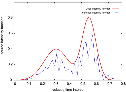For each case, we give the value of the identified source position and draw on the same figure the two curves showing the used intensity function introduced in (81) and the identified intensity function obtained from . We also give the relative error computed using (82).

The analysis of the numerical experiments presented in figures 1–4 shows that the established identification method enables to identify the elements defining the sought time–dependent point source with a relatively good accuracy. Those numerical results seem to be accurate and relatively stable with respect to the introduction of noises on the used measures.

Fig. 1 Noise intensity 3%: and ErrorLam = 13.43%.

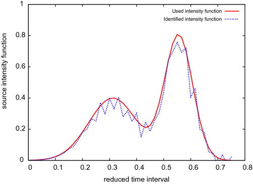
Fig. 2 Noise intensity 5%: and ErrorLam = 23.53%.

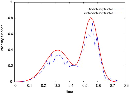
Fig. 3 Noise intensity 7%: and ErrorLam = 35.27%.

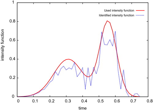
Fig. 4 Noise intensity 10%: and ErrorLam = 46.79%.

Furthermore, according to Step 2 we determine the source intensity function using the already identified source position in Step 1. Hence, a part of the error on the identified source intensity function comes from the error already committed on the computed source position. In practice, usually the suspect pollution source locations are rather known and the aim is to identify among all those suspect sources which one is the responsible of the observed accidental pollution and then, to recovery its loaded time-dependent intensity function. Therefore, Step 1 could lead to deduce the exact position of the sought source. Then, using rather than in Step 2 will improve the error .

Discussion and outlook

Note that the results established in this paper require the use of two observation points (sensors) which should frame the source region. The importance of this requirement can be easily seen from the stationary version of the underlined inverse source problem: In that case, we aim to identify the two unknown parameters and given some data measured by sensors. Then, for an explicit identification and since we have two unknowns, we need two measures. Furthermore, the analytic computation of the state reveals that it contains a term involving the Heaviside function at . Therefore, if the two needed measures are taken at the same side of the source position (both upstream or both downstream) then, the identification problem is equivalent to solving a system of two linearly dependent equations. Those two equations become linearly independent if one measure is taken upstream whereas the other is taken downstream with respect to the source position. That explains the need for two sensors and the fact that they should frame the source position. In practice, that seems to make sense since observing the source activity from only one side of the river will enable us to see some variation of the concentration but certainly not the significant change of its value between upstream and downstream regions. This significant change in the concentration represents the main characterization of the sought source.

As a work in progress, we are studying the robustness of the established identification method with respect to higher values of the Peclet number. This dimensionless number measures the ratio of the rate of advection by the rate of diffusion. The higher Peclet numbers correspond to the case of advection dominant flow. In such kind of flow, the damping effect exerted by the diffusion will be reduced and thus, from the engineering point of view, one expects more sensitivity on the signals recorded by sensors. Another interesting point of this work in progress is how to select the total number of discrete times . The value used in this paper was selected after numerous runs as the value of from which the accuracy of the identified results does not improve significantly anymore. According to our first observations, the value of seems depending on the Peclet number and thus, on the nature of the flow.

Conclusion

In this paper, we studied the identification of a time–dependent point source occurring in the right-hand side of a one-dimensional evolution linear transport equation with spatially varying diffusion, velocity and reaction coefficients. Under some reasonable conditions on those spatially varying coefficients and assuming the source intensity function vanishes before reaching the final control time, we proved the identifiability of the elements defining the sought time–dependent point source from recording the state at two observation points framing the source region. Then, we established an identification method that uses those records to localize the source position as the zero of a continuous and strictly monotonic function and transforms the task of recovering its intensity function into solving a deconvolution problem. Some numerical experiments on a variant of the water pollution model are presented. The analysis of those experiments shows that the established identification method is accurate and stable with respect to the introduction of noises on the used measures.

Proof of Proposition 5.1    For a constant velocity and a null reaction coefficient, the assertion (76) is equivalent to the main condition (15). And thus, according to Lemma 2.3, we have for all . Therefore, using (73) the function is defined on as follows:(82) where . In addition, according to (74), we find(83) Then, using the change of variable in (84) leads to(84) Now, by employing the change of variable in (85), we obtain(85) Hence, using (86) in (83) gives the result announced in (77).                      

Proof of proposition 5.2    The function that given associates is continuous and strictly increasing on . Then, using the change of variable we obtain(86) Therefore, from the last equality in (87), we find(87) Multiplying and dividing the left side of the first equality in (88) by giveswhich leads to(88) Since from (88) we have , then using (88) in (89) we obtain the result announced in (79).

References

- Xanthis, CG, Bonovas, PM, and Kyriacou, GA, 2007. Inverse problem of ECG for different equivalent cardiac sources, PIERS Online. 3 (2007), pp. 1222–1227.
- Koketsu, K, 2000. Inverse problems in seismology, bulletin of the Japan society for industrial and applied mathematics, Inverse Prob. 10 (2000), pp. 110–120.
- Baev, A, 2005. Solution of the inverse dynamic problem of seismology with an unknown source, Comput. Math. Model. 2 (2005), pp. 252–255.
- Cox, BA, 2003. A review of currently available in-stream water-quality models and their applicability for simulating dissolved oxygen in lowland rivers, Sci. Total Environ. 314–16 (2003), pp. 335–377.
- APHA. Standard methods for the examination of water and wastewater. 18th ed. Washington (DC): American Public Health Association. Bulut V.N..
- Fardin, B, and Mohammah, H, 2010. Pollution and water quality of the Beshar river, Engineering and Technology. 70 (2010), pp. 97–101.
- Linfield C, et al. The enhanced stream water quality models QUAL2E and QUAL2E-UNCAS: documentation and user manuel, EPA: 600/3-87/007; May 1987..
- Okubo, A, 1980. Diffusion and ecological problems: mathematical models. New York: Springer-Verlag; 1980.
- Lions, JL, 1992. "Pointwise control for distributed systems". In: Banks, HT, ed. Control and estimation in distributed parameters systems. Philadelphia, PA: SIAM; 1992.
- Badia, A, 2005. Ha Duong T, Hamdi A. Identification of a point source in a linear advection dispersion reaction equation: application to a pollution source problem, Inverse Prob. 21 (2005), pp. 1121–1136.
- Cannon, JR, 1968. Determination of an unknown heat source from overspecified boundary data, SIAM J. Numer. Anal. 5 (1968), pp. 275–286.
- Engl, HW, Scherzer, O, and Yamamoto, M, 1994. Uniqueness of forcing terms in linear partial differential equations with overspecified boundary data, Inverse Prob. 10 (1994), pp. 1253–1276.
- Yamamoto, M, 1993. Conditional stability in determination of force terms of heat equations in a rectangle, Mathl. Comput. Model. 18 (1993), pp. 79–88.
- Yamamoto, M, 1994. Conditional stability in determination of densities of heat sources in a bounded domain, Internat. Ser. Numer. Math. 18 (1994), pp. 359–370.
- Hettlich, F, and Rundell, W, 2001. Identification of a discontinuous source in the heat equation, Inverse Prob. 17 (2001), pp. 1465–1482.
- Badia, A, and Hamdi, A, 2007. Inverse source problem in an advection dispersion reaction system: application to water pollution, Inverse Prob. 23 (2007), pp. 2101–2120.
- Hamdi, A, 2009. Identification of a time-varying point source in a system of two coupled linear diffusion-advection-reaction equations: application to surface water pollution, Inverse Prob. 25 (2009), pp. 115009–115029.
- Hamdi, A, 2009. The recovery of a time-dependent point source in a linear transport equation: application to surface water pollution, Inverse Prob. 25 (2009), pp. 75006–75023.
- Dahlberg, B, and Trubowitz, E, 1984. The inverse Sturm-Liouville Problem III, Comm. Pure Appl. Math. 37 (1984), pp. 255–67.
- Kurbanov VM, Safarov RA. On uniform convergence of orthogonal expansions in eigenfunctions of Sturm-Liouville operator. Transactions of NAS of Azerbaijan. 2003:161–168..
- Jai, A, and Pritchard, G, 1988. Sensors and controls in the analysis of distributed systems. New York: Wiley; 1988.
- Bucur, A, 2006. About the second-order equation with variable coefficients, Gen. Math. 14 (2006), pp. 39–42.
- Titchmarsh, EC, 1937. Introducton to the theory of Fourier integrals. Oxford: Clarendon Press; 1937.
- Solodky, SG, and Mosentsova, A, 2008. Morozov’s discrepancy principle for the Tikhonov regularization of exponentially ill-posed problems, Comput. Methods Appl. Math. 8 (2008), pp. 86–98.
- Whitney, ML, 2009. Theoretical and numerical study of Tikhonov’s regularization and Morozov’s discrepancy principle [Mathematics Theses]. Atlanta, GA: Georgia State University; 2009.
- Rundell, W, and Sacks, P, 1992. Reconstruction techniques for classical inverse Sturm-Liouville problems, Math. Comput. 58 (1992), pp. 161–183.
- Veerle Ledoux. Study of special algorithms for solving Sturm-Liouville and Schroedinger equations [Ph.D. Thesis]. Ghent: Ghent University; 2007..
- Pérez Guerrero JS, Skaggs TH. Analytic solution for one-dimensional advection-dispersion transport equation with distance-dependent coefficients. J. Hydrol. 2010;390:57–65..
- Schwartz, L, 1966. Théorie des distributions. Paris: Hermann; 1966.