Crack identification in beams using Hilbert transform, kurtosis and mode shape rotation deviation curve

Abstract

An inverse problem of diagnosing cracks using empirical mode decomposition (EMD) and Hilbert transform (HT) is proposed based on theoretically obtained vibration data of classically supported structural beam elements. The procedure to obtain natural frequencies, mode shapes and dynamic response to excitation force of pristine and damaged beams is provided. Three different damage indices are used for detecting the crack, identifying the crack height and locating the damage. It is shown that intrinsic mode functions (IMFs), instantaneous frequency time (IF) and amplitude time (A) distributions extracted from dynamically acquired response signals are able to provide information about the existence and severity of crack. This study is the first in terms of (1) employing temporal and spatial signals along with HT, (2) presenting kurtosis usage for beams with different boundary conditions and (3) deriving the deviation curves for identifying the defects in structural beam elements. The proposed procedure and damage metrics are shown to be capable of detecting cracks as small as 4–5% of beam height, and are vigorous and noise robust.

Keywords:

• Euler–Bernoulli beam
• Hilbert transform
• empirical mode composition
• crack
• kurtosis
• mode shape rotation deviation curve

ASM Subject Classifications:

• 70J10
• 70J30
• 74H45
• 74R99

1. Introduction

Damage, if undetected at an early state, may pose a serious threat to the performance and integrity of structures that are of primary concern in many fields of engineering. A great number of research studies have been conducted to detect damages in the last three decades. Overall, structural damage detection methods can be categorized as local damage detection and global damage detection methods [1]. Local damage detection techniques such as X-ray and ultrasonic methods use only the data obtained from the damage structure, i.e. they do not require the base-line data and theoretical model of the undamaged structure. Though these methods have been the most common techniques in detecting damage on a structure [2] and have been very effective for small and regular structures, they are not suitable for large and complicated structures [3,4]34. For such structures, methodologies called global vibration-based damage detection have been proposed [5,6]56.

Being a hot spot in the inverse problem of structural damage diagnosis area, vibration-based methods can be divided into the traditional and modern methods [1] or modal or frequency-based and time-based methods [7]. The former types of detection methods are chiefly based on natural vibration characteristics of structures such as natural frequency and modal shape. The basic principle of these methodologies is that damages induce alteration in the dynamic properties that will eventually result in detectable changes in the modal properties of structures. For instance, the onset of crack leads to a reduction of natural frequencies and changes in modal shapes [8,9]89. The modal domain methods that have been dominant for the natural frequencies are rather easy to determine [10] and modal shapes contain local information, which makes them responsive to local damages [11]. Problems with modal domain, however, exist. Frequency changes are not very sensitive to small damages. Also, measurement errors degrade the ability of the methods to estimate the size of crack accurately [12]. The measurement of mode shapes requires a series of sensors. Additionally, environmental noise and choice of sensor locations noticeably affect the accuracy of the damage detection procedure [13].

The latter type of detection schemes is based on online-measured structural vibration responses to detect damage. Real-time monitoring of structures is performed by means of sensors embedded or mounted externally to the structure. Key factors to a successful monitoring and damage detection method are sensor technology and signal processing. Signal processing refers to extracting important features such as modal parameters of structures in time or frequency domain from the measured vibration signal [14]. Numerous approaches have been applied for this purpose [15,16]1516. Recently, a few new tools such as short-time Fourier transform (STFT), Wigner–Ville distribution (WVD), wavelet transform (WT) and Hilbert–Huang transform (HHT) providing both time and frequency information of a measured signal have been developed for the system identification and damage diagnosis. STFT is a moving-window Fourier transform. It assumes stationarity within each window and the window length and shape have to be chosen before the analysis. Due to uncertainty principle, there is a compromise between time and frequency solution [17]. To overcome the drawback of fixed window length, WT has been introduced as a windowing technique with a variable-sized region. VW, therefore, has been one of the most important and fastest evolving signal-processing tools in the last two decades [18]. WT is not, however, a real time-frequency analysis. In WT, similar to STFT, the mother wavelet has to be chosen and cannot be altered during the analysis [19]. WVD can describe the energy density of a signal simultaneously in both time and frequency. Hence, it can provide a high-resolution representation in time and frequency for non-stationary signals [20]. This merit is, on the other hand, overcome by such limitations as negative energies and non-linear behaviour [21]. It is derived that these methods have been designed for linear and non-stationary data. Unfortunately, in most real-life systems, the acquired data are most likely to be both non-stationary and non-linear. Recently, a new time-series method has been developed to analyse such non-linear and non-stationary behaviour [22]. This procedure consists of two parts. In the first part, the intrinsic mode functions (IMFs) of the obtained data are acquired through empirical mode decomposition (EMD). In the second part, time-frequency properties of IMFs are captured through Hilbert transform (HT) of the IMFs. Due to its ability to analyse non-linear and non-stationary data, the HT method has found many applications within the last decade. The following briefly presents the previous research pertinent to the structural damage detection via the integrated EMD and HT procedures.

Zhang et al. [23] used HT to evaluate structural damage from the vibration response based on the baseline measurements obtained from a pristine structural component. Li et al. [24] utilized HT to analyse the responses of as-built and rehabilitated bridge columns, and observed that at the instant the frequency changes, the structural behaviour changes from elastic to inelastic. Hence, it was concluded that the HT can be used to obtain the instantaneous natural frequencies of bridge columns. Yang et al. [25] proposed a method based on the HT to identify the system and detect the damage. The method was applied to the ASCE benchmark building model. Through only one measurement of the acceleration time history that may be polluted by noise, all the natural frequencies and damping ratios can be identified. Damages in the structure can be detected by comparing the stiffness of each story before and after damage scenario. ASCE benchmark problem was also studied by Yang et al. [26] to extract damage arouses due to a sudden change of structural stiffness from the measured data. The study also considered detecting damage time instants based on the EMD and HT. The benchmark problem was later studied by Liu et al. [27] to test the applicability of HT. The results showed that the HT method can detect and locate the structural damage and identify the instant of the impact loading of the damage taking place in the structure. The efficacy of the combined EMD and HT in locating an abnormality in the form of a crack, delamination, stiffness loss or boundary in beam and plate structure was shown by Quek et al. [28]. Physically obtained propagating wave signals were used for this objective. Chen et al. [29] established a dynamic model of one composite aircraft wingbox using ANSYS software and obtained the vibration responses of intact and damaged structures. The feature index vector of wingbox structure with different damage status was extracted for damage detection. In a recent study, Chiang et al. [30] examined the relationship between structural damage and sensitivity indices; the ratio of rotation, the ratio of shifting value, and the ratio of bandwidth, using the HT method. Roveri and Carcaterra [31] employed an HT method for damage detection of bridge structures under a travelling load. By a single-point measurement, the presence and location of the damage along the beam were identified.

Most of the research studies dealing with damage diagnosis through the EMD and HT in the current literature have been carried out for such structures as buildings, bridges, plates, or mechanical components. The vibration data are obtained from a single or multiple locations and analysed by means of a signal-processing technique. Those research works regarding beam-type structures have mainly used the wave propagation signals to infer damage characteristics. To the authors’ knowledge, there are no literature studies on the HT-based methods for health monitoring of classically supported beam-type structures via dynamic data acquired from a single point. This is the first aim of the study herein. The EMD- and HT-based research has mostly considered moderate and large size of cracks in the range of 0.10–0.40% of the element height. Even, in one study, it was shown that the HT procedure is not sensitive to crack height [31]. Yet, the cracks of these sizes are readily detected by traditional procedures such as frequency-based methods. Moreover, the detection of smaller-sized cracks has been reported in the literature. For instance, cracks as small as 4% of beam height with measurement noise present are identified based on stationary wavelet transform (SWT) of the mode shape data [32]. This sets the second aim of this paper: to examine the effectiveness of EMD and HT technique to diagnose small cracks present on beam-type structures. Besides, the detection of damage and its size, the third objective of this study, is to determine the geometric location of the damage. From the dynamically acquired data, the exact location of a crack cannot be determined. One of the most commonly used procedures for this purpose is to utilize modal shape data, which contain local information that makes them more sensitive to local damages. The mode shape and mode shape rotation data are obtained as spatial-domain signals in the study, which are then subjected to HT in order to identify the damage by noticing the local discontinuity in the HT elements. The statistical parameter kurtosis is also applied to localize the crack. Kurtosis values are determined from the mode shape and mode shape rotation data of undamaged and damaged beams. Any kurtosis value greater than the one corresponding to the undamaged case presents an indication of incipient crack. Finally, the present study derives the mode shape deviation and mode shape rotation deviation curves (MSRDCs) to locate the crack and to determine the crack height. The deviation curves are generated from modal shape data through a simple transformation. The efficiency and sensitivity of the above schemes are investigated for a wide range of crack ratios of 0.005–0.50 present on classically supported beams. The beams are modelled using Euler–Bernoulli beam theory having a single crack. The proposed study, however, can be readily extended to include multiple cracks.

2 The Hilbert–Huang transform

Proposed by Huang et al. [22], the transform consists of EMD and Hilbert spectral analysis. In the first stage, a vibration signal is decomposed into a collection of IMFs. IMFs satisfy the following two conditions: (1) in the whole data-set, the number of extrema and the number of zero crossings must either equal or differ at most by one; and (2) at any point, the mean value of the envelope defined by the local maxima and the envelope defined by the local minima is zero. The IMFs represent the vibration modes embedded within the signal where each IMF contains only one mode of oscillation with no complex riding waves present.

The decomposition is performed through a repeated sifting procedure. This procedure is briefly described as follows. Connect all the local maxima by a cubic (or higher order) spline as the upper envelope and connect all the local minima by a cubic spline as the lower envelope. Calculate the mean of the envelopes and subtract it from the time series. This procedure is repeated until the mode function meets the above IMF requirements. The result is the first component. Subtract the first IMF from the original time signal and work on the residue using the same procedure until the second IMF is extracted. Repeat this process until the residue is too small to be of significant consequence or becomes a monotonic function from which no more IMFs can be obtained. At the end, the time signal x(t) can be expressed in terms of n number of IMFs:(1) $x(t)=\sum _{j=1}^n{c}_j(t)+r_n(t)$(1) where $c_j(t)$ is the jth IMF component and $r_n(t)$ is the residue. In the second stage, the HT is utilized to obtain phase and frequency information. Having determined time series $c_j(t)$, their HT is defined as(2) $y_j(t)=\text{H}[c_j(t)]=\frac{1}{\pi }{\int }_{-\infty }^{+\infty }\frac{c_j(\tau )}{t-\tau }d\tau$(2) which implies that the analytical signal becomes(3) $z_j(t)=c_j(t)+{\mathit{iy}}_j(t)=a_j(t)e^{i{\theta }_j(t)}$(3) where $i=\sqrt{-1}$ and(4) $a_j(t)=\sqrt{c_j^2(t)+y_j^2(t)}\text{,}{\theta }_j(t)=\text{atan}\frac{y_j(t)}{c_j(t)}$(4)

In this equation, a_j is the instantaneous amplitude and θ_j is the instantaneous phase function. By the virtue of the IMFs, the concept of time varying frequency and phase angle has substantial meaning. The instantaneous circular frequency can then be defined as(5) ${\omega }_j(t)=\frac{\mathrm{d}{\theta }_j(t)}{\mathrm{d}t}$(5)

After performing the HT on each IMF component, the original data x(t) can be retrieved as the real part of the complex expression as(6) $x(t)=\mathfrak{R}\left[\sum _{j=1}^n{a}_j(t)e^{i\int {\omega }_j(t)\mathrm{d}t}\right]$(6) which enables to represent the amplitude and instantaneous frequency as functions of time.

In the implementation of the HT method, one needs to pay attention to (1) obtaining the signal characteristics correctly, (2) the criterion for ending the sifting process and (3) spline-fitting problems. The EMD method sometimes may not disclose the signal characteristics properly due to the mode mixing effect. Mode mixing displays that vibrations of different time scales reside in one IMF component or vibrations of the same time scale in different IMF components. A remedy to overcome the mode mixing separation problem is given in [33]. The second problem arises when a stringent criterion to terminate the sifting process is used to obtain IMFs. Excessive sifting can shatter the physical sense of frequency and amplitude modulations. Quek et al. [28] proposed the normalized standard deviation between two consecutive siftings. The last problem is caused when the spline fit results in large swings at the ends of the signal. The discrepancy between the spline and original signal may subsequently propagate inward and corrupt the signal [29]. A MATLAB code is written in this study, which implements the above solutions. The developed code is tested against the routines freely available online and realized to give much improved results.

3 Structural damage indices

The presence of damage, its location, its size and the prediction of the remaining service life of a structure are the various hierarchical targets to reach for any damage detection scheme. A damage index or metric is the key tool to infer any information about the damage [34]. Therefore, a proper damage feature index needs to be constructed in order to detect damage by using structural dynamic response signals. The index should meet the following two requirements: the metric must be sensitive to structural local damage and it must be monotone function of the location coordinate [35].

Due to the ability of the HT method to extract embedded oscillations, to disclose hidden reflections in the data and to accurately describe the frequency content through a high-resolution energy time-frequency representation, virtually all components of HT have been exploited in the literature as damage indices. Depending on the analysis and structure type under investigation, the index can be a local or global measurement or a direct visual comparison of any HT elements corresponding to pristine and cracked states. For instance, Chen et al. [29] used the absolute maximum of relative error of normalized instantaneous frequency values as a local index to detect damages in composite wingboxes. Li et al. [2] utilized the relative energy character rate as a global metric to identify damage occurrence time in a shear building model. Mahgoun et al. [33] visually compared the IMF components to see the influence of ensemble EMD and to detect early damage in rotating machines. In this study, the root mean square error (RMSE) is employed as an index to measure the differences between the intact and cracked beam responses. This measure of differences is widely used in various fields of engineering but never been resorted to in the HT-based signal-processing methods. RMSE can be expressed as the difference between the values of intact and damaged structures squared and then averaged over the time history, i.e.(7) ${\text{RMSE}}_j=\sqrt{\frac{\sum _{i=1}^N({\widehat{\alpha }}_{j\text{,}i}-{\alpha }_{j\text{,}i}{)}^2}{N}}$(7) where N is the length of vibration signal, ${\alpha }_{j\text{,}i}$ and ${\widehat{\alpha }}_{j\text{,}i}$ are the HT-based IMF, instantaneous frequency (IF) or amplitude (A) of intact and cracked beams, and the subscripts j and i refer to the corresponding order of HT component and time, respectively. RMSE is a global index that takes into account the deviations from the healthy case over the whole time history of each IMF, IF or A components. Therefore, this index is not affected by local jumps in the HT components that may result from errors like end effects.

In the last step of this study, the location of crack is determined using (1) the HT. Since the dynamically acquired data cannot be used for this purpose, mode shape and mode shape rotation of the damaged beam will be utilized. The modern damage detection schemes such as WT have been applied to mode shape data in the current literature. However, mode shape change data have never been used in conjunction with the HT method. In this study, the data obtained from the cracked beams alone will be taken as spatial domain signal and fed into the HT to locate the crack. (2) Kurtosis. In statistics, kurtosis is a measure of the peakedness of the probability distribution of real-valued random variable. Higher kurtosis means more of the variance due to infrequent extreme deviation. It is given by(8) $\kappa =\frac{\sum _{i=1}^N[\varphi (k)-\mu {]}^4}{(N-1){\sigma }^4}$(8) where {$\varphi (k)$} is a sequence, μ is the mean of {$\varphi (k)$}, σ is the standard deviation and N is the number of data points. This parameter has been used for detection of defects in bearings [36], gearbox [37] and cantilever beam [38]. To the authors’ knowledge, this study is the first to use kurtosis in an HT-related study. (3) Mode shape and MSRDCs. This index is derived from the work of Babu and Sekhar [39] who presented a new procedure called slope deviation curve (SDC). This curve is generated from Operational Deflection Curve (ODC), which is completely different from mode shapes. ODC is obtained from the motion of two or more points on a structure subjected to a dynamic loading. For the beam-type structures utilized in this study, the SDC did not yield steady results, from which the location of crack can be identified. Therefore, a new deviation curve scheme is proposed here. The deviation curves are generated from already available fundamental mode shape and mode shape rotation data and, hence, called mode shape deviation curve (MSDC) and MSRDC. They are determined by a simple transformation. Let ${\varphi }_i$ (${\varphi }_i^{\prime }$) be the ith datum of fundamental mode shape (rotation) along the beam. Then,(9) ${\overline{\varphi }}_i={\varphi }_{i+1}-{\varphi }_i({\overline{\varphi }}_i^{\prime }={\varphi }_{i+1}^{\prime }-{\varphi }_i^{\prime })$(9) is determined. Plotting these data vs. their location yields the deviation curves.

4 Cracked beam modelling

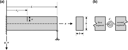
Beams with four different end conditions are considered in this study. The beams are modelled utilizing Euler–Bernoulli beam theory. Figure 1 shows a model of uniform beam with a crack. The x-coordinate is along the length of the beam and y is along the height of the beam. v is the transverse displacement of the beam. L is the beam length. The crack is modelled by massless rotational spring. The additional flexibility induced by the presence of crack is defined by the local compliance C which causes a jump in the slope of the beam at that location.

Figure 1 (a) Model of beam with a crack and (b) rotational spring model connecting two beam segments.

The governing differential equation for the free flexural vibration of intact Euler–Bernoulli beam [40] is(10) $\frac{{\partial }^{4}v(x\text{,}t)}{\partial x^4}+\frac{\overline{m}}{K_b}\frac{{\partial }^{2}v(x\text{,}t)}{\partial t^2}=0$(10) where K_b = EI is the flexural stiffness, E is the Young’s modulus of elasticity, I is the area moment of inertia, $\overline{m}=\rho A$ is the mass per unit length, $\rho$ is the mass density and A is the area of beam cross-section. Assuming the variation of transverse deflection of the beam at any location to be(11) $v(x\text{,}t)=\varphi (x)e^{i\omega t}$(11)

Equation (10) becomes(12) $\frac{d^4\varphi (x)}{{\mathit{dx}}^4}-\frac{\overline{m}{\omega }^2}{K_b}\varphi (x)=0$(12) where $i=\sqrt{-1}\text{,}$ ω and $\varphi (x)$ are the circular frequency and mode-shape function of the beam, respectively.

The general form of the solution for Equation (12) is given by(13) $\varphi (x)=D_1{S}_1(x)+D_2{S}_2(x)+D_3{S}_3(x)+D_4{S}_4(x)$(13) where D_j (j = 1, 2, 3, 4)’s are constants to be determined from the boundary conditions and S_j’s are the linearly independent solutions: $S_1(x)=\sin (\mathit{kx})$, $S_2(x)=\cos (\mathit{kx})$, $S_3(x)=\sinh (\mathit{kx})$, and $S_4(x)=\cosh (\mathit{kx})$ with $k=\sqrt[4]{\overline{m}{\omega }^2/K_b}$. To simplify the analysis of vibration of the Euler–Bernoulli beam, the linearly independent fundamental solutions denoted by ${\overline{S}}_j(x)(j=1\text{,}2\text{,}3\text{,}4)$ are constructed. This is done by satisfying the normalization condition at the origin of axes (see for details, [41]). Consequently, the following are obtained(14) $\begin{array}{c}\hfill {\overline{S}}_1(x)=\frac{1}{2}\cos (\mathit{kx})+\frac{1}{2}\cosh (\mathit{kx})\hfill \\ \hfill {\overline{S}}_2(x)=\frac{1}{2k}\sin (\mathit{kx})+\frac{1}{2k}\sinh (\mathit{kx})\hfill \\ \hfill {\overline{S}}_3(x)=-\frac{1}{2k^2}\cos (\mathit{kx})+\frac{1}{2k^2}\cosh (\mathit{kx})\hfill \\ \hfill {\overline{S}}_4(x)=-\frac{1}{2k^3}\sin (\mathit{kx})+\frac{1}{2k^3}\sinh (\mathit{kx})\hfill \end{array}$(14)

Using the above solutions for ${\overline{S}}_j$’s, the mode-shape of the first segment ($0\le x<x_1$) can be formulated as(15) ${\varphi }_1(x)=\varphi (0){\overline{S}}_1(x)+{\varphi }^{\prime }(0){\overline{S}}_2(x)-\frac{M(0)}{K_b}{\overline{S}}_3(x)-\frac{V(0)}{K_b}{\overline{S}}_4(x)$(15) where $\varphi (0)\text{,}{\varphi }^{\prime }(0)\text{,}M(0)$ and $V(0)$ are the displacement, rotation, moment and shearing force of the beam at $x=0\text{,}$ respectively. Only two of these parameters are unknown for any type of support conditions. The compatibility conditions enforce the continuity of the force and displacement fields across the crack. For a crack located at section $x_1\text{,}$ these conditions can be expressed as(16) $\begin{array}{c}\hfill {\varphi }_2(x_1)={\varphi }_1(x_1)\hfill \\ \hfill V_2(x_1)=V_1(x_1)\hfill \\ \hfill M_2(x_1)=M_1(x_1)\hfill \\ \hfill {\varphi }_2^{\prime }(x_1)={\varphi }_1^{\prime }(x_1)+C_1{\varphi }_1^{″}(x_1)\hfill \end{array}$(16) where C₁ is the compliance of the cracked section. The expressions in Equation (16) show the equalities of displacement, shear force, bending moment and rotation, respectively, at the common interface of the first segment and the second segment of the beam. C₁ can be expressed as(17) $C_1=5.346·h·f(a_1/h)$(17) where h is the height of the beam cross section and a₁ is the depth of the crack. The function $f(a_1/h)$ is the dimensionless local flexibility computed from the strain energy function and given by(18) $\begin{array}{c}\hfill f(a_1/h)=1.862(a_1/h{)}^2-3.95(a_1/h{)}^3+16.375(a_1/h{)}^4-37.226(a_1/h{)}^5+76.81(a_1/h{)}^6\hfill \\ \hfill -126(a_1/h{)}^7+172(a_1/h{)}^8-143.97(a_1/h{)}^9+66.56(a_1/h{)}^{10}\hfill \end{array}$(18)

The mode-shape function for the section ($x_1\le x<L$) after the crack can be determined based on Equations (17) and (18) as(19) ${\varphi }_2(x)={\varphi }_1(x)+C_1{\varphi }_1^{″}(x_1){\overline{S}}_2(x-x_1)H(x-x_1)$(19) in which $H(·)$ is the Heaviside function, which assumes 0 for $x<x_1$ and 1 for $x\ge x_1$. The characteristic equation is readily established by imposing boundary conditions on the above equation. This is outlined next for beams with classical two-end supports.

4.1 Fixed–fixed beam

If the beam is fixed at both ends, the compatibility requirements are(20) $\varphi (0)=0\text{,}{\varphi }^{\prime }(0)=0\text{and}\varphi (L)=0\text{,}{\varphi }^{\prime }(L)=0$(20)

Then the mode shape of the first segment ($0\le x\le x_1$) becomes(21) ${\varphi }_1(x)=\left[-\frac{{\overline{S}}_3(x)}{K_b}\right]M(0)+\left[-\frac{{\overline{S}}_4(x)}{K_b}\right]V(0)\text{.}$(21)

Using Equations (19)–(21), one obtains:(22) $\left[-\frac{{\overline{S}}_3(L)}{K_b}-C_1\frac{{\overline{S}}_3^{″}(x_1)}{K_b}{\overline{S}}_2(L-x_1)\right]M(0)+\left[-\frac{{\overline{S}}_4(L)}{K_b}-C_1\frac{{\overline{S}}_4^{″}(x_1)}{K_b}{\overline{S}}_2(L-x_1)\right]V(0)=0$(22) (23) $\left[-\frac{{\overline{S}}_3^{\prime }(L)}{K_b}-C_1\frac{{\overline{S}}_3^{″}(x_1)}{K_b}{\overline{S}}_2^{\prime }(L-x_1)\right]M(0)+\left[-\frac{{\overline{S}}_4^{\prime }(L)}{K_b}-C_1\frac{{\overline{S}}_4^{″}(x_1)}{K_b}{\overline{S}}_2^{\prime }(L-x_1)\right]V(0)=0$(23)

Setting the second-order determinant consisting of the coefficients of M(0) and V(0) in Equations (22) and (23) to zero gives the characteristic equation, from which the Eigen frequencies can be consequently determined. Substituting the calculated value of ω_j into Equations (22) and (23), and setting one of M(0) and V(0) equal to 1 or any other value, one determines the jth modal shape. Having computed the modal shape, the determination of mode shape rotation is elementary.

4.2 Fixed-hinged beam

For a fixed-hinged beam, the Eigen function of the first segment is given by Equation (21). Support conditions for the right end are(24) ${\varphi }_2(L)=0\text{,}{\varphi }_2^{″}(L)=0$(24)

Using Equations (19), (21) and (24) yields Equation (22) and the following:(25) $[{\overline{S}}_2^{″}(L)+C_1{\overline{S}}_2^{″}(x_1){\overline{S}}_2^{″}(L-x_1)]\varphi (0)+\left[-\frac{{\overline{S}}_4^{″}(L)}{K_b}-C_1\frac{{\overline{S}}_4^{″}(x_1)}{K_b}{\overline{S}}_2^{″}(L-x_1)\right]V(0)=0$(25)

Since Equations (22) and (25) contain only two unknowns (i.e. V(0) and M(0)), a second-order determinant consisting of the coefficients of V(0) and M(0) is obtained. Setting the determinant to zero, the frequency equation is determined.

4.3 Fixed-free beam

The mode-shape function of the first segment of the beam is also given by Equation (21). If the beam is free at the right end,(26) ${\varphi }_2^{″}(L)=0\text{and}{\varphi }_2^{‴}(L)=0$(26) are obtained. These conditions results in Equation (25) and the following:(27) $\left[-\frac{{\overline{S}}_3^{‴}(L)}{K_b}-C_1\frac{{\overline{S}}_3^{″}(x_1)}{K_b}{\overline{S}}_2^{‴}(L-x_1)\right]M(0)+\left[-\frac{{\overline{S}}_4^{‴}(L)}{K_b}-C_1\frac{{\overline{S}}_4^{″}(x_1)}{K_b}{\overline{S}}_2^{‴}(L-x_1)\right]V(0)=0$(27)

The frequency equation can be implemented by setting the second-order determinant that consists of the coefficients of M(0) and V(0) in Equations (25) and (26) equal to zero.

4.4 Simple–simple beam

The boundary conditions for a simply-supported beam are given by(28) $\varphi (0)=0\text{,}M(0)=0\text{and}\varphi (L)=0\text{,}M(L)=0$(28)

Substituting the expressions in Equation (28) into Equation (15), one obtains the mode-shape of the first segment of the beam as(29) ${\varphi }_1(x)=[{\overline{S}}_2(x)]{\varphi }^{\prime }(0)+\left[-\frac{{\overline{S}}_4(x)}{K_b}\right]V(0)\text{.}$(29)

Using Equations (19), (28) and (29) leads to(30) $[{\overline{S}}_2(L)+C_1{\overline{S}}_2^{\prime \prime }(x_1){\overline{S}}_2(L-x_1)]\varphi (0)+\left[-\frac{{\overline{S}}_4(L)}{K_b}-C_1\frac{{\overline{S}}_4^{\prime \prime }(x_1)}{K_b}{\overline{S}}_2(L-x_1)\right]V(0)=0$(30) (31) $[{\overline{S}}_2^{″}(L)+C_1{\overline{S}}_2^{″}(x_1){\overline{S}}_2^{″}(L-x_1)]\varphi (0)+\left[-\frac{{\overline{S}}_4^{″}(L)}{K_b}-C_1\frac{{\overline{S}}_4^{\prime }(x_1)}{K_b}{\overline{S}}_2^{\prime }(L-x_1)\right]V(0)=0$(31)

Equations (30) and (31) can be rewritten in a matrix form. Since there are only two unknowns, the size of coefficient matrix becomes 2 × 2. Setting the determinant of the matrix to zero, the frequency equation is established.

Once the mode shapes and frequencies have been determined utilizing the above equations, the dynamic response of the beams under a point loading can be computed using the mode-superposition analysis [42], which is quite familiar to the engineering community. Hence, the details are not given here.

5 Results

Four classically-supported beam-type structures are studied. The beams are subjected to a sinusoidal loading at x = 0.2L. The crack is introduced to the beam at a location x₁ = 0.4L. The crack heights of 0.005h to 0.50h are considered. The beam properties are: b = h = 0.10 m, L/h = 10, E = 7 × 10¹⁰ N/m², ρ = 2780 kg/m³. As stated previously, frequency-based methods are traditionally favoured as the natural frequencies can be conveniently measured from just a few points on the beam. Therefore, the feasibility of natural frequency changes in identifying the damage will be first evaluated. Table 1 lists the relative frequency errors between the pristine and damaged beams. Among the four cases of beam types, the results of the fixed–fixed beam are shown since being the stiffest, the fixed–fixed beam is more affected by the introduction of a crack. Results in the table show that the variation of relative frequency errors is very small as compared to the variation of crack height. It is acknowledged that it is necessary for a natural frequency to change about 5% in order for the damage to be detected [43]. Hence, the cracks in such beam structures cannot be determined by utilizing the natural frequency variations. A similar comparison is made between the mode shapes of undamaged and damaged beams. The results, not shown here, also indicated that the mode shapes are not very sensitive to the cracks.

Table 1. Ratios of the first five modal frequencies of intact and damaged fixed–fixed beam with varying crack depths.

	$(f_0-f_i)/f_0$
a/h	Mode 1 (%)	Mode 2 (%)	Mode 3 (%)	Mode 4 (%)	Mode 5 (%)
0.005	0.002	0.000	0.000	0.002	0.000
0.02	0.021	0.014	0.007	0.037	0.000
0.05	0.124	0.098	0.054	0.221	0.003
0.10	0.462	0.379	0.194	0.802	0.012
0.20	1.687	1.355	0.699	2.756	0.042
0.30	3.635	2.836	1.470	5.413	0.084

Figure 2 shows the time history responses acquired at a location x = 0.7L of the intact and damaged beam having a crack with ratio of 10%. Again, no obvious difference can be seen between the two time-domain response signals. Consequently, the response signals are decomposed via EMD into their IMF components, which are then subjected to the HT to yield instantaneous frequency–time (IF) and amplitude–time (A) distributions. From the IMF, IF and A distributions, not supplied here for brevity, one cannot note at a glance the differences between the two cases, especially for beams with small cracks. Therefore, RMSE values between the intact and cracked beam response signals are computed. Tables 234 show those values determined from IMF, IF and A distributions, respectively. It is noted that the acquired response signals yield five IMF components. For very small cracks (a/h = 0.005), the errors are close to zero but as the crack height increases, RMSE values also increase. Generally, the differences between the first components are the largest. However, the second or the third components may be dominant for large crack sizes (see, for instance, the RMSE values of IMF component for a/h = 0.175). This suggests that an aggregate error estimate would be reasonable by combining the component-based errors. Since there are several error measurements (5 in this case) and no component has a real major dominance, utilizing Root-Sum-of-Squares (RSS) is meaningful [44]. Error estimates for each component is squared, they are added and then square root is taken. The corresponding values are given in the last column of Tables 234. It is seen now that as the crack severity increases, the RSS values systematically increase, indicating strongly the existence of damage. The RMSE or RSS values being small, one may argue that these values may be buried in the changes caused by environmental or operational conditions. It is generally assumed that the variations due to environmental effects and ambient vibration can be as high as 5–10%. Therefore, the proposed error index needs to be tested against noise. A noise with zero mean and unit standard deviation is added to the pristine beam response as follows:(32) $x_{\text{noise}}(t)=x(t)+y_{\text{noise}}(t)\times \mathit{SF}\times \mathit{RMS}(x(t))$(32) where x_noise(t) is the response signal with noise, x(t) is the original signal obtained from the pristine beam, y_noise(t) is the randomly generated noise vector with zero mean and unit standard deviation, SF is the scale factor (or noise level), and the RMS(x(t)) is the root-mean-square value of x(t). In this study, a noise level of 5% due to previously explained rationale is examined. Table 5 shows the error estimates between the original signal and contaminated signal. By comparing the last column of this table with those of Tables 234, it is noticed that one can detect cracks as small as 4–5% of the beam height present in beam-type structures with the proposed damage metric.

Figure 2 Displacement responses at x = 0.7L of fixed–fixed intact beam and damaged beam with a crack ratio of 0.10.

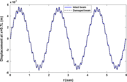
Table 2. RMS errors of IMF components and RSS values of fixed–fixed beam.

a/h	IMF1	IMF2	IMF3	IMF4	IMF5	RSS
0.005	0.00001	0.00001	0.00000	0.00000	0.00001	0.00002
0.01	0.00001	0.00000	0.00000	0.00000	0.00000	0.00001
0.02	0.00003	0.00002	0.00001	0.00001	0.00001	0.00004
0.05	0.00017	0.00004	0.00001	0.00001	0.00002	0.00018
0.08	0.00041	0.00009	0.00002	0.00006	0.00000	0.00042
0.10	0.00063	0.00009	0.00001	0.00000	0.00003	0.00064
0.125	0.00096	0.00013	0.00001	0.00002	0.00001	0.00097
0.15	0.00144	0.00061	0.00021	0.00021	0.00013	0.00160
0.175	0.00184	0.02958	0.03550	0.00510	0.01329	0.04839
0.20	0.00231	0.02877	0.03932	0.01483	0.01401	0.05287

Table 3. RMS errors of IF components and RSS values of fixed–fixed beam.

a/h	IF1	IF2	IF3	IF4	IF5	RSS
0.005	0.00012	0.00000	0.00001	0.00000	0.00000	0.00012
0.01	0.00013	0.00000	0.00000	0.00000	0.00000	0.00013
0.02	0.00023	0.00001	0.00001	0.00000	0.00000	0.00023
0.05	0.00106	0.00001	0.00001	0.00000	0.00000	0.00106
0.08	0.00212	0.00002	0.00014	0.00000	0.00000	0.00212
0.10	0.00450	0.00001	0.00002	0.00000	0.00000	0.00450
0.125	0.00648	0.00003	0.00000	0.00000	0.00000	0.00648
0.15	0.01733	0.00028	0.00041	0.00000	0.00000	0.01734
0.175	0.03209	0.03936	0.00219	0.00005	0.00000	0.05083
0.20	0.02974	0.09109	0.00411	0.00004	0.00000	0.09591

Table 4. RMS errors of A components and RSS values of fixed–fixed beam.

a/h	A1	A2	A3	A4	A5	RSS
0.005	0.00001	0.00001	0.00000	0.00000	0.00001	0.00002
0.01	0.00000	0.00000	0.00000	0.00000	0.00000	0.00000
0.02	0.00002	0.00002	0.00000	0.00001	0.00001	0.00003
0.05	0.00004	0.00004	0.00001	0.00001	0.00002	0.00006
0.08	0.00007	0.00008	0.00001	0.00007	0.00000	0.00013
0.10	0.00009	0.00010	0.00001	0.00001	0.00003	0.00014
0.125	0.00013	0.00015	0.00001	0.00003	0.00001	0.00020
0.15	0.00056	0.00063	0.00017	0.00029	0.00014	0.00092
0.175	0.00054	0.03066	0.04459	0.00686	0.01295	0.05607
0.20	0.00064	0.03100	0.05033	0.02085	0.01374	0.06417

Table 5. RMS errors of IMF, IF, and A components and RSS values between the responses of intact beam and the same response with 5% noise.

	Component number
	1	2	3	4	5	RSS
IMF	0.00002	0.00003	0.00002	0.00002	0.00002	0.00005
IF	0.00041	0.00001	0.00003	0.00000	0.00000	0.00041
A	0.00002	0.00003	0.00003	0.00003	0.00002	0.00006

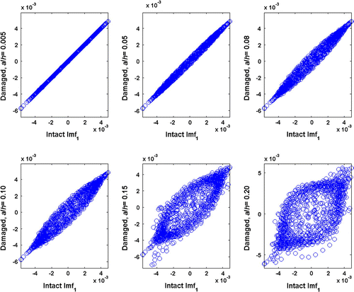
The efficiency of the EMD and HT is next investigated by a direct visual comparison. Scatter diagrams are used for this purport. The diagrams are obtained by plotting the IMF values (IF or A values) of the intact beam on the horizontal axis and plotting those of the damaged beam on the vertical axis. Figures 345 show such scatter charts of IMF, IF and A components, respectively, for a damaged beam with a 5% crack ratio. It is observed that, in the scatterplots of components except the first component, a line with unit slope is obtained, suggesting no significant variation between the IMF and instantaneous values of intact and damaged beams. However, the first components show an obvious variation for the cracked beam with a/h = 0.05. It would be of interest to see the scatterplots for other crack ratios to examine the deviations from the line having a unit slope. Figure 6 shows the scatter charts of the first IMF components for crack heights of 0.05h–0.20h. The effect of larger cracks is clearly observed in this figure. Similar figures are also obtained for instantaneous frequency and amplitude distributions but not shown here.

Figure 3 Scatter diagrams of IMFs corresponding to intact and damaged beam with a crack ratio of 0.05.

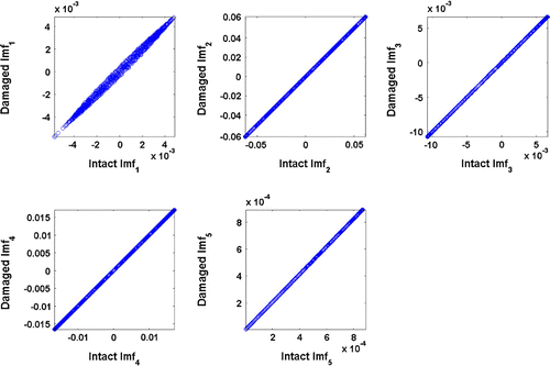
Figure 4 Scatter diagrams of IFs corresponding to intact and damaged beam with a crack ratio of 0.05.

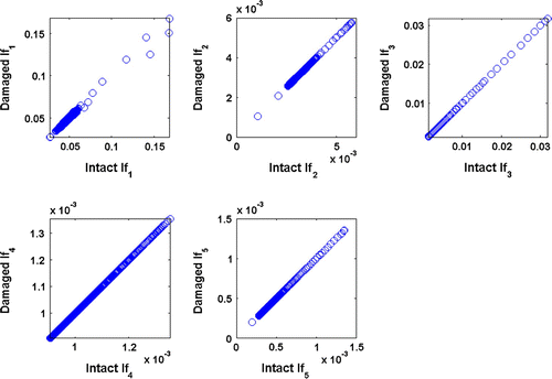
Figure 5 Scatter diagrams of A corresponding to intact and damaged beam with a crack ratio of 0.05.

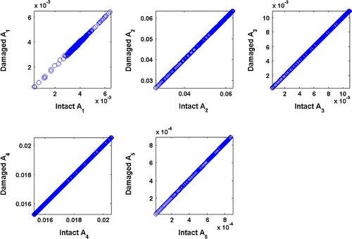
Figure 6 Scatter diagrams of IMFs corresponding to intact and damaged beams with crack ratios of 0.005, 0.05, 0.08, 0.10, 0.15 and 0.20.

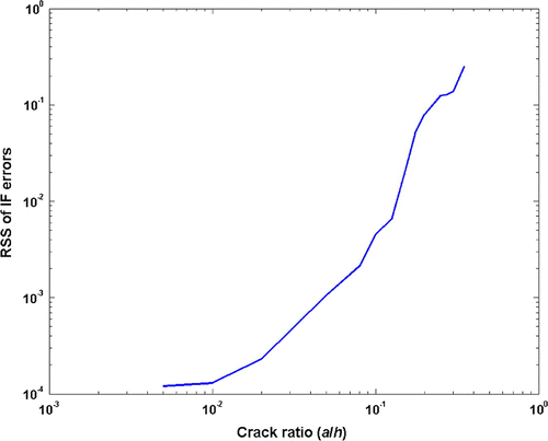
Having determined the existence of damage, the estimation of crack depth is next studied. Formerly computed RSS quantities of IMF, IF or A components may be used for this intent. Figure 7 shows the log–log plot RSS values based on the IF errors vs. normalized crack depths varying from 0.5 to 35% (a maximum crack height of 0.35h is used as the response signals acquired from the beam with larger crack sizes yield 6 HT components, obstructing the comparison with those five components of the intact beam). The RSS values increase with crack size according to an almost second-order polynomial. This, hence, enables an estimation of crack size.

Figure 7 Crack ratios vs. RSS of IF errors for fixed–fixed beam with a crack.

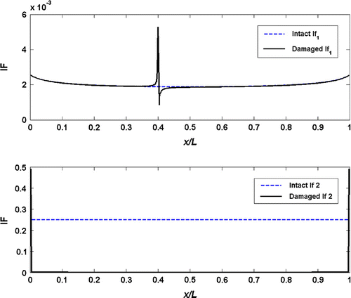
Determination of crack location is considered in this part of the study. The response signal acquired at a single point on the beam cannot be used with the HT to identify the crack location. Mode shape and mode shape rotation data, already determined during the time history analysis, are employed for this purpose. These data are treated as spatial domain signal and utilized along with the HT. Figure 8 shows the IF of the fundamental mode shape of fixed–fixed intact beam and damaged beam with a crack ratio of 5% located at x₁ = 0.4L. Since the mode shape is an IMF itself, it generates one component only. The figure displays for the cracked beam an irregularity at the crack location. The IF vs. the data points along the beam length is shown in Figure 9 for the intact and damaged beam with a crack ratio of 20%. The irregularity at the crack location is now more apparent, implying that the transformation of modal shapes through the HT may be used to identify the crack location. However, the IMF and A transformations of the mode shapes do not result in any irregularities and as a result; they cannot be used for detection of the damage location. Figures1011 display the IFs of mode shape rotations against the beam length. Note that the mode shape rotation data produce two components, the second component being the residue though. These transformations also produce distortions at the crack location. They, thus, may be used for the determination of crack location as well. The use of mode shape rotation data has one advantage: their A transformations also indicate the crack location. The corresponding A plots are not supplied here for brevity.

Figure 8 Instantaneous frequencies from the transform of mode shape data of a fixed–fixed beam with a/h = 0.05.

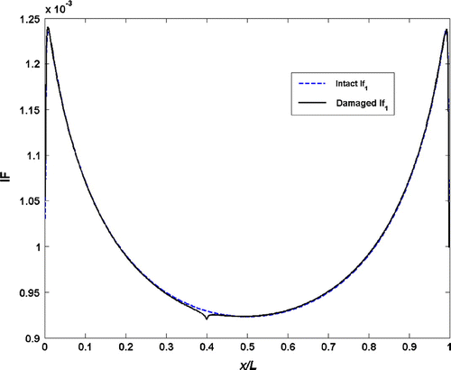
Figure 9 Instantaneous frequencies from the transform of mode shape data of a fixed–fixed beam with a/h = 0.20.

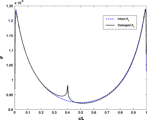
Figure 10 Instantaneous frequencies from the transform of mode shape rotation data of a fixed–fixed beam with a/h = 0.05.

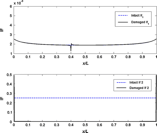
Figure 11 Instantaneous frequencies from the transform of mode shape rotation data of a fixed–fixed beam with a/h = 0.20.

The kurtosis is a measure of the heaviness of the tails in the distribution of $\varphi (k)$ $(k=1\text{,}\dots \text{,}N)$ sequence in Equation (8). Abrupt changes in the sequence have high values and consequently appear in the tails of the distribution. These high values in the kurtosis parameter enable it to be used as a statistical metric in identifying the existence of crack in beam structures. 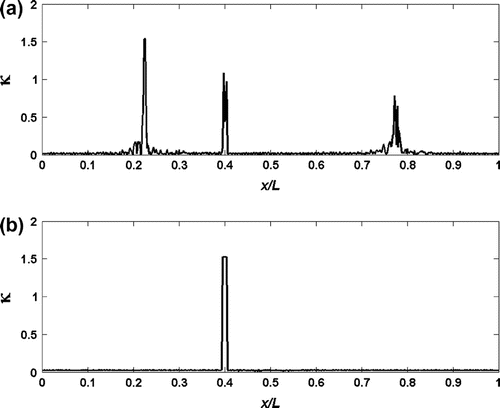The spatial domain signal $\varphi (k)$ (${\varphi }^{\prime }(k)$) considered in this study is the mode shape (mode shape rotation) data corresponding to the fundamental mode, which is the most readily measured mode of vibration. Using Equation (8) for the whole beam length, provides a single value of kurtosis index that does not give any particular information about the crack location. Therefore, the kurtosis should be computed at a more local level by utilizing a windowed signal instead of the whole signal. The length of the windowed signal M is much smaller than the length of the mode shape data N. For each M-sample data, one kurtosis value is computed and the M-sample window is right shifted. This scheme is repeated until the end of N-sample of spatial domain signal. Point-to-point values of kurtosis are obtained, through which the exact point of crack location is captured. The outlined process is applied to the mode shape and mode shape rotation signals using a window length of M = 7. The obtained kurtosis values along the spatial coordinates are given in Figure 12(a) and (b), respectively. The spatial data are obtained from fixed–fixed beam with a crack height of 0.05h. The crack is located at x₁ = 0.4L. Figure 12(a) displays three regions of abrupt changes, one of which is the crack location. Hence, the use of mode shape signal blurs the exact crack location. On the other hand, the kurtosis plot of mode shape rotation signal gives exactly the crack location. The process is applied to other crack sizes and different beam types and, hereby it is realized that in all the cases studied, the kurtosis plots captured the crack location.

Figure 12 Kurtosis estimates determined from (a) mode shape and (b) mode shape rotation data of a fixed–fixed beam having a crack with height ratio of 0.05.

Lastly, the MSDC and MSRDC are investigated as to their efficacy in detecting the crack on beam-type structures. The deviation curves are obtained from a simple transformation of the fundamental mode shape information, as explained in Equation (9). They are presented in Figure 13 for a fixed–fixed beam having a crack of varying depth. It is seen that the MSDCs ($\overline{\varphi }$) do not generate any information regarding the crack location whereas the MSRDCs (${\overline{\varphi }}^{\prime }$) accurately shows the existence of crack at the prescribed location. It is noted that the abrupt changes in ${\overline{\varphi }}^{\prime }$ increase with the increase in crack ratios. This variation, hence, may be used to assess the crack severity. 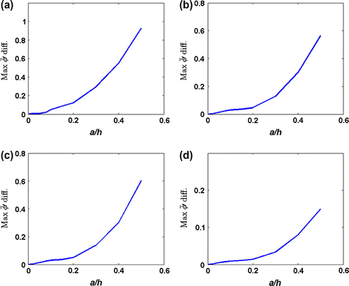The changes in ${\overline{\varphi }}^{\prime }$ values vs. the crack sizes are shown in Figure 14 for all the beam types considered in this study. It is clearly seen from the figures that the maximum differences obtained in ${\overline{\varphi }}^{\prime }$ values increase with an increase in crack height. Note that differences in ${\overline{\varphi }}^{\prime }$ values of fixed–fixed beam are the largest as, being the stiffest, the fixed–fixed beam is the most affected by the same crack size. The variations of ${\overline{\varphi }}^{\prime }$ values with respect to the crack height in all four plots of Figure 14 may be expressed as a second-order polynomial, which can be consequently employed for crack diagnose.

Figure 13 Mode shape deviation and MSRDCs for cracked fixed–fixed beam with crack ratios of (a) 0.05, (b) 0.10, (c) 0.20 and (d) 0.50.

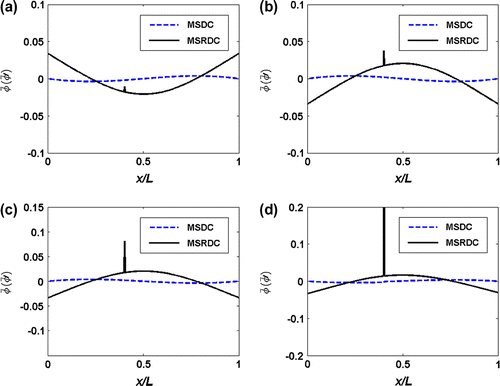
Figure 14 Variations in MSRDCs with respect to crack height for (a) fixed–fixed, (b) fixed–hinged, (c) simple–simple and (d) fixed–free beam.

6 Conclusions

A model-based damage detection method using EMD and HT has been proposed in this study to identify the location and severity of damage on beam-type structures. A comprehensive parametric study considering different boundary conditions of beam elements and varying crack ratios is performed for this purpose. The conclusions drawn can be briefly summarized as follows:

• The comparison of natural frequencies, mode shapes and dynamically acquired response signals of intact and cracked beams do not provide any information regarding the existence of crack unless the crack size is large.

• Application of HT to response signals yields IMF, instantaneous frequency and amplitude distributions. The RMSEs between these HT components of pristine and damaged beams indicate the presence of crack. The efficiency of the RMSE-based damage index is tested against noise. It is shown that cracks as small as 4–5% of the beam height can be detected via the proposed damage index.

• RSS of the errors determined from the HT elements may be used to quantify the level of crack.

• The efficiency of the developed HT algorithm is also shown visually through the use of scatter diagrams.

• The localization of crack is performed by utilizing the mode shape and mode shape rotation of fundamental mode of vibration. These data are used as spatial domain information and transformed using HT. The instantaneous frequency transformation of mode shape reveal the location of crack while both the instantaneous frequency and amplitude transformation of mode shape rotation give the location of damage.

• Kurtosis of mode shape rotation also clearly shows the location of crack whereas kurtosis of mode shape masks the exact location of damage.

• Mode shape deviation and MSRDCs are obtained from a simple conversion of modal shape data. Although the MSRDC presents abrupt changes in the crack location, MSDC presents no information regarding the crack location. This indicates once again the superiority of the use of mode shape rotation as a damage index over the use of mode shape.

• Employing the abrupt changes, one can relate the size of crack to the magnitude of alteration occurring in the MSRDC. Consequently, this relationship is shown to follow a second-order polynomial law.

The results presented demonstrate that HT is a suitable tool for processing non-stationary response signals encountered in damage detection research studies. The IMF, instantaneous frequency and amplitude distributions determined from the response time histories provide a good realization of existence of crack on beam-type structures. The same distributions obtained from the mode shape rotation spatial signal, statistical kurtosis value and MSRDC of the fundamental mode of vibration supply clear information about the crack location. Yet, the results of this study need to be verified experimentally. This study can be easily extended to consider multiple cracks on structural beam elements.

References

- Yan YJ, Cheng L, Wu ZY, Yam LH. Development in vibration-based structural damage detection technique. Mech. Syst. Signal Pr. 2007;21:2198–2211.
- Li H, Xiaoyan D, Hongliang D. Structural damage detection using the combination method of EMD and wavelet analysis. Mech. Syst. Signal Pr. 2007;21:298–306.
- Carden EP, Fanning P. Vibration based condition monitoring: a review. Struct. Health Monit. 2004;3:355–377.
- Auweraer HV. International research projects on structural damage detection. Key Eng. Mater. 2001;204:97–112.
- Shi ZY, Law SS, Zhang LM. Structural damage detection from modal strain energy change. J. Eng. Mech. ASCE. 2000;126:1216–1223.
- Gawronski W, Sawicki JT. Structural damage detection using modal norms. J. Sound Vib. 2000;229:194–198.
- Fan W, Qiao P. Vibration-based damage identification methods: a review and comparative study. Struct. Health Monit. 2011;10:83–111.
- Masoud A, Jarrad MA, Al-Maamory M. Effect of crack depth on the natural frequency of a prestressed fixed–fixed beam. J. Sound Vib. 1998;214:201–212.
- Narkis Y. Identification of crack location in vibrating simple supported beams. J. Sound Vib. 1993;172:549–558.
- Morassi A. Crack-induced changes in Eigen-parameters of beam structures. J. Eng. Mech. ASCE 1993;119:1798–1803.
- Farrar CR, James GH. System identification from ambient vibration measurements on a bridge. J. Sound Vib. 1997;205:1–18.
- Kim TJ, Stubbs N. Improved damage identification method based on modal information. J. Sound Vib. 2002;252:223–238.
- Kim TJ, Ryu YS, Cho HM, Stubbs N. Damage identification in beam-type structures: frequency-based method vs. mode shape-based method. Eng. Struct. 2003;25:57–67.
- Speckmann H, Daniel JP. Structural health monitoring for airliner, from research to user requirements, a European view. Monterey, CA: Conference on Micro-Nano-Technologies; 2004.
- Doebling SW, Charles RF. The state of the art in structural identification of constructed facilities. American Society of Civil Engineers Committee on structural identification of constructed facilities; 1999.
- Jiang X, Adeli H. Dynamic fuzzy wavelet neural network for nonlinear identification of highrise building. Comput. Aided Civ. Inf. 2005;20:316–330.
- Kim I, Lee H, Kim J. Impact damage detection in composite laminates using PVDF and PZT sensor signals. J. Intel. Mater. Syst. Str. 2005;16:1007–1013.
- Abbate A, DeCusatis CM, Das PK. Wavelets and subbands: fundamentals and applications. Boston, MA: Birkhauser; 2002.
- Kijewski T, Kareem A. Wavelet transforms for system identification in civil engineering. Comput. Aided Civ. Inf. 2003;18:339–355.
- Debnath L. Wavelet transforms and their applications. Boston, MA: Birkhauser; 2002.
- Polyshchuck VV, Choy FK, Braun MJ. New gear-fault-detection parameter by use of joint time–frequency distribution. J. Propul. Power. 2000;16:340–346.
- Huang NE, Shen Z, Long SR, Wu MC, Shih HH, Zheng Q, Yen NC, Tung CC, Liu HH. The empirical mode decomposition and the Hilbert spectrum for nonlinear and non-stationary time series analysis. Proc. R. Soc. Lond. A. 1998;454:903–995.
- Zhang RR, King R, Olson L, Xu Y. A HHT view of structural damage from vibration recordings. San Diego, CA: Processings of ICOSSAR; 2001.
- Li YF, Chang SY, Tzeng WC, Huang K. The pseudo dynamic test of RC bridge columns analyzed through the Hilbert–Huang transform, 13th world conference on earthquake engineering. BC: Vancouver; 2004.
- Yang JN, Lin S, Pan S. Damage identification of structures using Hilbert–Huang spectral analysis, 15th ASCE engineering mechanics conference. New York: Columbia University; 2002.
- Yang JN, Lei Y, Lin S, Huang N. Hilbert–Huang based approach for structural damage detection. J. Eng. Mech. ASCE 2004;130:85–95.
- Liu J, Wang X, Yuan S, Li G. On Hilbert–Huang transform approach for structural health monitoring. J. Intel. Mater. Syst. Str. 2006;17:721–728.
- Quek ST, Tua PS, Wang Q. Detecting anomalies in beams and plate based on the Hilbert–Huang transform of real signals. Smart Mater. Struct. 2003;12:447–460.
- Chen HG, Yan YJ, Jiang JS. Vibration-based damage detection in composite wingbox structures by HHT. Mech. Syst. Signal Pr. 2007;21:307–321.
- Chiang WL, Chiou DJ, Chen CW, Tang JP, Hsu WK, Liu TY. Detecting the sensitivity of structural damage based on the Hilbert–Huang transform approach. Eng. Comput. 2010;27:799–818.
- Roveri N, Carcaterra A. Structural health monitoring using empirical mode decomposition and AM/FM demodulation. The international conference surveillance 6. Compiegne; 2011.
- Zhong SC, Oyadiji SO. Crack detection in simply supported beams without baseline modal parameters by stationary wavelet transform. Mech. Syst. Signal Pr. 2007;21:1853–1884.
- Mahgoun H, Felkaoui A, Bekka RE. The effect of resampling on the analyses results of ensemble empirical mode decomposition (EEMD). The international conference surveillance 6. Compiegne; 2011.
- Rytter A. Vibration based inspection of civil engineering structure. Denmark: Aalborg University, Ph.D. diss.; 1993.
- Yan YJ, Hao HN, Yam LH. Vibration-based construction and extraction of structural damage feature index. Int. J. Solids Struct. 2004;41:6661–6676.
- Prabhakar S, Mohanty AR, Sekhar AS. Application of discrete wavelet transform for detection of ball bearing race faults. Tribol. Int. 2002;35:793–800.
- James LC, Limmer JD. Model-based condition index for tracking gear wear and fatigue damage. Wear. 2000;241:26–32.
- Hadjileontiadis LJ, Douka E, Trochidis A. Crack detection in beams using kurtosis. Comput. Struct. 2005;83:909–919.
- Babu TR, Sekhar AS. Detection of two cracks in a rotor-bearing system using amplitude deviation curve. J. Sound Vib. 2008;314:457–464.
- Weaver W, Timoshenko SP, Young DH. Vibration problems in engineering. New York: Wiley; 1990.
- Li QS. Vibratory characteristics of multi-step beams with an arbitrary number of cracks and concentrated masses. Appl. Acoust. 2001;62:691–706.
- Clough RW, Penzien J. Dynamics of structures. New York: McGraw-Hill; 1993.
- Salawu OS. Detection of structural damage through changes in frequency: a review. Eng. Struct. 1997;19:718–723.
- Taylor JR. An introduction to error analysis: the study of uncertainties in physical measurements. Sausalito, CA: University Science Books; 1997.