Abstract
The paper presents a study of solution of inverse medium scattering problems for time-harmonic electromagnetics in 3D. The solution is based on minimization of the misfit function between the observed scattered waves and trial solutions of direct problems for the sought approximate distribution of electric permittivity. The sources of illuminating waves and the observation points of the scattered fields are located in the vicinity of the scatterer. The simulations of the direct problems are performed with the adaptive finite element method. Tests with real- and complex-valued distributions of electric permittivity, and with complete and incomplete measurement data are presented.
Introduction
Inverse medium scattering problems in electromagnetics consist in evaluating the of electromagnetic material parameters, (possibly) complex-valued electric permittivity or magnetic permeability
of a material body from measurements of scattered electromagnetic waves due to known illuminations. The procedure has many potential applications including medical tomography, localization of burried objects, detection of material defects etc. The advantage of the so-called microwave tomography in medical applications would be its non-invasive character, the significant contrast of
for tissues with medical condition like a tumor, low cost and easy access. Obviously, we expect that the resolution of the method could not be as good as the resolution of the X-ray or magnetic resonance imaging techniques. Yet, the aforementioned advantages might make the method very useful for early detection of the decease.
Algoritms for solving inverse medium scattering problems in electromagnetics were investigated by Vögeler,[Citation1] Bao and Li,[Citation2] Hohage,[Citation3] Bulyshev et al.,[Citation4] Fhager et al. [Citation5] and other researchers. The techniques proposed by Vögeler, Bulyshev and Fhager were also applied for real-life measurements. The approach proposed in this work is similar to the method of Bulyshev and his co-workers. It consists of minimization of a misfit function between the measured scatterd fields and simulated scattered waves for trial distributions of electric permittivity. We follow this idea but we differ in approximation of solutions of direct and inverse problems. We also have broaden the class of problems by considering non-homogeneous backgrounds.
Fig. 1 Scattering problem of electromagnetics.
The present work is a continuation of paper [Citation6]. The new contribution includes the aforementioned problems with non-homogeneous backgrounds, both scattered and total field formulations for direct problems, illuminations generated by finite dipoles located inside a computational domain and consistent application of perfectly matched layer (PML) technique to truncate the computational domain.
A closely related problem of elastic inverse scattering was investigated in works of Epanomeritakis et al., [Citation7] Plessix,[Citation8] Virieux and Operto.[Citation9]
Scattering problem
We consider the classical problem of scattering a time-harmonic incident electromagnetic wave with a bounded obstacle. The electromagnetic field satisfies the time-harmonic Maxwell equations.(2) where
and
denote the electric and magnetic fields,
is the impressed current,
is the imaginary unit and
is the circular frequency. Parameters
and
are the complex electric permittivity and magnetic permeability. In this work,
and
, where
and
are the electric permittivity and conductivity (for simplicity, throughout this work we use the system of units in which the electric permittivity and magnetic permeability of the free space,
). A common approach is to eliminate one of the fields, e.g.
, to obtain the reduced wave equation for the electric field:
(3) In scattering problems, we look for a perturbation of a prescribed incident electric field
caused by placing in the free space a non-homogeneous dielectric object, see Figure . This perturbation is called the scattered field
. Since the total electric field,
, satisfies the reduced wave Equation (2.2) and the incident field satisfies a version of (2.2) with
in
, the scattered field
must satisfy the following equation:
(4) provided the material is non-magnetic,
, the case for biological tissues.
We can look for the solution of Equation (2.3) in a bounded domain by assuming that the Dirichlet and Neumann traces of the scattered field,
and
, (where
is the wavenumber) are related by the Dirichlet-to-Neumann,
-operator
of the unbounded domain
[Citation10].
(5) which can be approximated using the boundary element method (BEM), the PML technique,[Citation11] infinite elements (IE) or impedance boundary conditions.[Citation12] By multiplying the wave Equation (2.3) with a test function
, integrating it over domain
and integrating by parts the term with second derivatives, we end up with the following variational formulation: find
such that
(6) with
and
denoting the following bilinear and linear forms:
(7) where
is the characteristic impedance of the free space. Alternatively, we may obtain the weak statement for the total field formulation (2.2) (with
) for which the bilinear form
coincides with (2.6)
and functional
is as follows:
(8) The least expensive approximation of the
-operator can be expressed by the impedance condition
(9) The technique suffers, however, from an irreducable modelling error unlike the IE or BEM techniques.
Fig. 2 Finite element mesh of elements of order p=2 with the enriched layers to approximate the solution in PML.
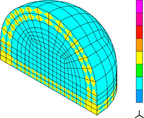
The PML technique has an advantage over the above methods that it can be used not only for scattering in a free space but also in a layered medium. The method consists of replacing the true electric permittivity and magnetic permeability
by the corresponding tensors
and
characterizing orthotropic medium with damping properties in relatively thin layers surrounding the computational domain with compact sources. The solution rapidly decays in the layer and we can impose a homogeneous Dirichlet boundary condition on the external boundary of the layer Footnote1. For rectangular, cylindrical and spherical layers, the distribution of
and
can be designed in such a way that the exact solution of the scattering problem with PML is identical with the exact solution in the whole space. The only problem is to approximate accurately enough the rapidly decaying waves in the PML. We can do this, for instance, by appropriate enrichment of the FE mesh. An example of a FEM mesh of order
with layers of elements of the order enriched to
(in the radial direction) for approximation of a decaying solution in PML is shown in Figure . The tensors of electric permittivity and magnetic permeability in PML take the following form:
(10) where for cylindrical PML
(11) while for the spherical PML
(12) where
and
are the basis vectors of the cylindrical and spherical coordinates, respectively. In the above formulas,
and
are complex-valued functions of the cylindrical coordinates
or spherical coordinate
, respectively. They are designed to provide smooth decay of the waves in PML. These so-called ‘complex stretch functions’ in this work are selected as
(13) where
is the internal radius of PML,
is its thickness and
. Outside PML
. The definition of
is analogous except that we must distinguish the upper and bottom PML of the cylinder.
The weak formulation for both scattered and total fields with PML is analogous to formulations discussed above in (2.6) and (2.7) though we neglect the presence of the -operator
.
Inverse medium scattering problem
The inverse medium scattering problem consists in reconstructing the distribution of material parameters characterizing the medium, in our case , based on observation of the scattered waves corresponding to some prescribed incident fields. We assume that both sources of incident waves and receivers are located in a vicinity of the scatterer. This is motivated by the desire to construct a method close to possible practical applications.
The set-up of the inverse problem is as follows. We consider the sources of illuminating waves (transmitters) and observation points of the scattered field (receivers) located at a finite and small distance from the scatterer. Transmitters are modelled with dipoles and assumed to be distributed almost uniformly over a sphere of radius containing the scatterer or, alternatively, over a half of this sphere. We consider
incident waves
and
observation points
. The incident field radiated by a dipole takes form [Citation13]:
(14) where
is the moment of the dipole,
location of the point relative to the dipole,
and
.
As an alternate way of generating illuminating waves, we also consider the following local distribution of the impressed current (in cylindrical coordinates):(15) where
, and
is the location relative to the centre of the antenna. The support of
is contained in a sphere of radius
. The distribution is axisymmetric, and smooth,
-continuous. We distribute these sources of waves analogously as pointwise dipoles, however, they are located inside the computational domain. We use
as a source of waves in the case when the scatterer is located in the medium consisting of two half-spaces with different electric permittivities. For this case, a closed formula for the field of the radiating dipole is not known so that illuminating waves must be found numerically. This can be easily done for the smooth
as opposed to the pointwise dipole.
The scattered field at the observation point outside of computational domain
is evaluated based on the equivalence principle and using the following representation formula [Citation14]:
(16) where
is the Green function for the scalar Helmholtz equation,
, and
is any surface surrounding the scatterer (or point
in a homogeneous space). We note that components of
are linear functionals.
At each observation point , we measure the scattered fields
due to incident waves
. We look for a distribution
by minimizing the discrepancy between the measured
and the simulated
corresponding to trial distributions
Footnote2:
(17) Trial distributions
are approximated by a linear combination of trilinear FE shape functions
, on an auxiliary mesh covering a selected subdomain
, outside of which
:
(18)
, where
is an a priori known domain containing the scatterer.
The optimization is performed with the deterministic technique, the quasi-Newton Broyden–Fletcher–Goldfarb–Shanno (BFGS) method in the implementation of Zhu, Byrd and Nocedal [Citation15]. It allows one to account for the natural constraints and
. We evaluate gradient of functional
using the method of adjoint problem (see for instance Petryk and Mróz [Citation16]) to be discussed next.
The adjoint problem
We recall the idea to evaluate using the adjoint problem. Let us first state the way parameters
enter the problem in bilinear form
and linear functional
:
(19) (for the total field formulation (2.7)
is independent of
). For simplicity, let us consider first the case of a real-valued weak formulation (
,
,
and
are real-valued). We consider an augmented real-valued functional
(20) where
plays the role of the Lagrangian multiplier and a test function. We investigate a variation of
due to an infinitesimal perturbation
of parameters
.
(21) where, following (3.17), we have
(22) (for the total field formulation (2.7)
) and the two of indicated terms in (4.20) vanish due to the weak formulation for
and due to the condition to be stated in (4.22). Namely, we define the solution of the adjoint problem as a solution of the following weak statement: find
such that
(23) Therefore, with this choice of
, we find that the gradient of L can be expressed as:
(24) Now, we remove the restriction that the form
is real-valued. We note that the weak formulation of electromagnetics is in a way redundant. The following three conditions are equivalent
(25) This lets us choose the third option of the above to define the real-valued augmented functional with
as follows:
(26) and evaluation of
must be modified accordingly. It should be emphasized that solution of the adjoint problem adds no significant computational burden because the forward and adjoint formulations share the same stiffness matrix which is decomposed only once.
Finite element discretization
Solutions of direct problems in are approximated using the FEM with hexahedral edge elements. We use the FE code with a capability of
-refinements. That is, we can selectively subdivide elements reducing their size
and non-uniformly change their spectral orders
.[Citation12] Both operations can be anisotropic. In this work, we typically use elements of order
and we only use the
capability to enrich locally the order of approximation. The unbounded computational domain can be truncated using approximation of the
-operator of the external domain with the IE, boundary element method, absorbing boundary conditions or PML technique. The last approach is favoured in this work as, in prospect, it will allow us to model a part of the human body adjacent to the rest of the body.
The systems of linear equations resulting from the FEM discretization are solved with the direct solver MUMPS [Citation17] using eight processors.
Numerical examples
Our motivation of solving inverse medium scattering problems is the possibility of reconstructing the distribution of the complex electric permittivity from the measurements of scattered fields. Such distribution would provide a three-dimensional image of the scatterer. A frequently used procedure of investigating inverse problem solution algorithms is to use numeriacally simulated measurements. That is, we obtain numerically the scattered fields at measurement points for the prescribed distribution of
and we perturb them to mimic the measurement errors. This is also our way of running tests.
The antennas are distributed over a sphere of radius . Their distribution is close to uniform and it is obtained as follows. We subdivide the sphere into six identical quadrilateral patches bounded by six planes
. For each patch we consider two families of
intermediate planes between the separating planes, rotated by the angle of
. Intersections of planes of both families and the sphere define locations of antennas. The number of these points is
for
. We assume that each transmitter is a source of waves of two mutually orthogonal polarizations tangential to the sphere. In actual tests it was sufficient to use
, i.e. 26 receivers/transmitters and 52 illuminating waves.
We solve the test problems with real- and complex-valued distributions of . We also consider the tests with the measurement data obtained for points spread over the entire surface surrounding the scatterer, and the tests based on measurements obtained on a half of the sphere. We refer to these two situations as the complete and incomplete data cases. For the incomplete case, we use larger density of antennas taking parameter
which results in
antennas spread over a hemisphere. The measurement perturbation is of the form
with rand
being a uniformly distributed random number, and
is the amplitude of the noise. In majority of tests
. We recover
in subdomains
which concide with supports of
except for the last test with substantially larger
.
We use the waves of the free space wavelength (only in the first example
). In other words, the unit of length is
. In all tests, optimization required less than 100 solutions of direct problems, and the rough image of the inverse solution was recognizable after 10–20 optimization steps. The size of the direct problems did not exceed 200,000 d.o.f. Thus, using the MUMPS solver and an 8-node workstation, we could obtain a rough solution in about 10 min and a converged solution in about one hour. We expect this could be substantially accelerated.
Two Gaussian hills
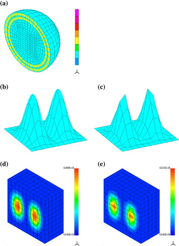
We consider the following distribution of real-valued electric permittivity:(27) where
(28) Similar distribution was investigated by Bao and Li [Citation2]. Figure presents the finite element mesh with 141,700 d.o.f. We solved the problem in a ball of radius
. It is truncated by the PML of the thickness
. The distribution of
is reconstructed in
, we use 729 variables for approximation of
. The incident waves are generated by 26 dipoles located on a sphere of radius
where we also put the 26 measurement points. The exact and reconstructed distributions of
are shown in Figure . Accuracy of the recovered
was
% in the
-norm. We used the scattered field formulation.
Fig. 3 Two Gaussian Hills scatterer. (a) FE mesh, (b), (d) exact and (c), (e) reconstructed real-valued electric permittivity .
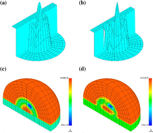
Kidney-like scatterer
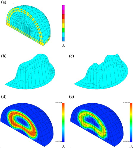
In this test, we consider the real-valued and incomplete scattering data (the antennas are located on the northern hemisphere). The distribution of electric permittivity is defined as follows:
(29) where
is a Hermite polynomial such that
. The function above is extended to 3D by rotational symmetry w.r.t.
-axis, i.e. by substitution
. The contours of
resemble the shape of a kidney. The scatterer is placed in the computational domain
in the form of an upper half of a ball of radius
extended by a cylindrical part at the bottom. It is truncated by the PML of the thickness
.
The incident waves are radiated by the dipoles located on the upper hemisphere of radius , i.e. inside
, and we use the scattered field formulation. The scattered field at the measurement points (coinciding with the dipoles) is evaluted via formula (3.15) with
being a boundary of the domain bounded by the spheres of radii 2 and 3 and the
-plane. This might seem unnatural as the direct solution is known at any point inside
. However, a linear functional defined as a pointwise value of the solution,
, is not continuous in the
-norm and it could not be used as the load functional for the adjoint problem. The value of the scattered field as expressed by the integral formula (3.15) does not suffer this drawback (in fact, in this situation, we may consider formula (3.15) as some kind of post-processing of FEM solution).
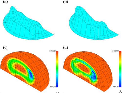
The exact and reconstructed distributions of are shown in Figure . We reached the accuracy of 11%. We used a FE mesh with 160,200 d.o.f. and 1448 variables to approximate
.
Fig. 4 Kidney-like scatterer (a) FE mesh, (b),(d) exact and (c),(e) reconstructed real-valued electric permittivity .
Kidney-like scatterer with a tumor
We consider the distribution of complex-valued electric permittivity . The real part is defined as in (6.28) while the imaginary part,
. In addition, we modify these distributions by local bumps – ‘tumors’ that we define as follows:
(30) where
and
is the central point of the tumor,
is its radius. Parameter
defines the contrast of the perturbation. Function
is modified only if
. We set
and
for the real part and
and
for the imaginary part. In this example, we use the incomplete data. The transmitters and receivers are located on the upper hemisphere of radius 2.5 inside
. This was motivated by the desire to mimic the possible conditions of medical examination (for instance of a breast).
The transmitters are modelled by the localized impressed currents as defined in (3.14), with -axis corresponding to one of two directions of polarizations. We use the total field formulation. The finite element mesh of ndof = 120,000 is a little coarser than in the previous example. The exact and recovered electric permittivity are presented in Figures and . We observe satisfactory resolution of the ‘tumors’ in the reconstructed image. In this problem, we used 2064 real-valued d.o.f. to approximate the distribution of electric permittivity and 15% accuracy of
was reached.
Fig. 5 Kidney-like scatterer with tumors. (a),(c) exact and (b),(d) reconstructed real part of complex electric permittivity .
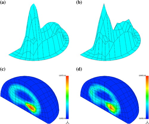
Fig. 6 Kidney-like scatterer with tumors. (a),(c) exact and (b),(d) reconstructed imaginary part of complex electric permittivity .
Breast-like scatterer with a tumor
In our next example, we consider scattering on an object located in the medium consisting of two half-spaces of different electric properties, separated by the horizontal plane. In the upper half-space while in the bottom one
. The scatterer occupies the upper half-ball of radius
and it is adjacent with its basis to the plane separating the two half-spaces. The distribution of
is specified as follows:
(31) where
is the Hermite polynomial as in (6.28). The contours of
are half-circles. In addition, as in the previous example, we add local perturbations, bumps–tumors (6.29), that we define by the following parameters: for the real part
and
, and for the imaginary part
and
.
Fig. 7 Scatterer with tumors in two half-spaces. (a) FE mesh, (b) location of smeared dipoles.
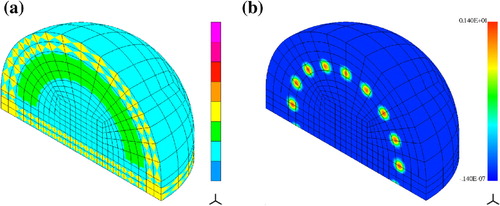
Both, the sources of incident waves and observation points are located on a northern hemisphere of radius 2.5 inside the computational domain. We use the local impressed currents as defined in (3.14) as the transmitters, Figure shows their locations – the distribution of . In fact they were designed just for this kind of problems as we do not know the closed formula for the field of a radiating dipole in a two half-spaces medium. Also for this reason, the direct problems are solved using the total field formulation. To improve the accuracy of direct solutions in the region of smeared dipoles, we enriched the order of approximation to
in this area. The FE mesh of 155,600 d.o.f. is shown in Figure . The evaluation of the scattered field was performed as in the previous test. We present the exact and reconstructed distributions in Figures and . As before satisfactory resolution of the local perturbations of
is observed. The accuracy of
was reached and we used 2418 real-valued d.o.f. to approximate the inverse solution. Comparing to the previous tests, we had to reduce the amplitude of random perturbation of the simulated measurements to
to obtain the acceptable quality of the inverse solution. Larger perturbations were causing deterioration of reconstructed
, not affecting much
. This effect requires further investigation.
The example discussed above reflects a procedure of examination of a female breast with medical condition, with the two half-spaces modelling the human body and the free space.
Fig. 8 Scatterer with tumors in two half-spaces. (a), (c) exact and (b),(d) reconstructed real part of complex electric permittivity .
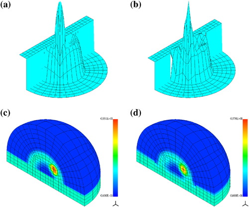
Fig. 9 Scatterer with tumors in two half-spaces. (a),(c) exact and (b),(d) reconstructed imaginary part of complex electric permittivity .
Limb-like scatterer with tumors
In the next example, we consider scattering on an elongated object resembling a limb with internal structure of two ‘bones’ and two tumors. The distribution of is specified as follows
(32) where
and
, while the imaginary part,
(33) We added two tumors analogously as before with the following parameters (compare definition (6.29)):
We tried to reconstruct the distribution of
in a cylinder of radius
and height
. Figure shows the FE mesh with ndof = 171,800 and distribution of the antennas: there are eight smeared dipoles on each of five equidistant levels around the cylinder (locations of observation points are identical). That is we use 40 sources of radiating waves with two polarizations, i.e. the total of 80 illuminating waves. The mesh is enriched to
in the region with smeared dipoles to enable approximation of rapidly varying fields. The inverse solution was approximated using 1552 real-valued d.o.f.
Fig. 10 Limb-like scatterer with tumors: (a) FE mesh, (b) location of antennas.
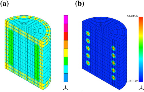
Fig. 11 Limb-like scatterer with tumors: (a),(c) exact and (b),(d) reconstructed
.
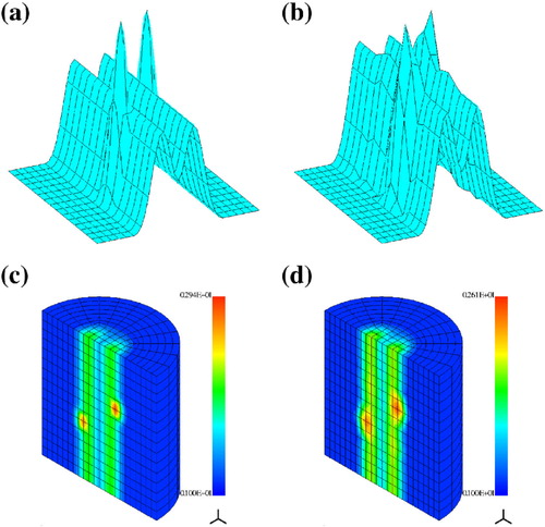
Fig. 12 Limb-like scatterer with tumors: (a),(c) exact and (b),(d) reconstructed
.
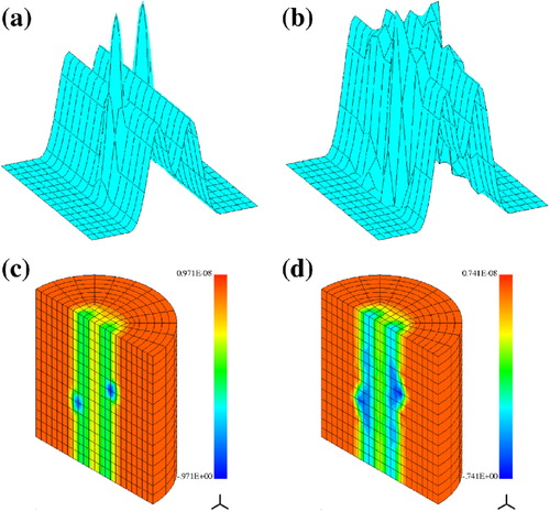
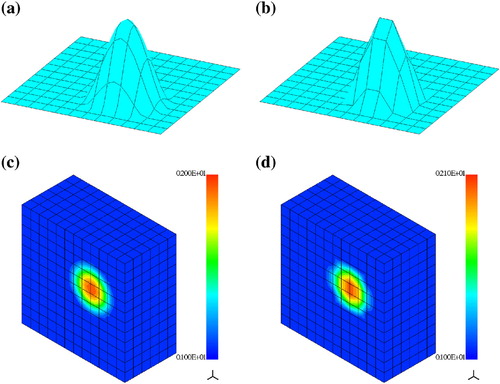
Fig. 13 Localized scatterer. (a), (c) exact and (b), (d) reconstructed real-valued electric permittivity .
Evaluation of the scattered field is performed as in example Section26.2 with the integration surface being the boundary of a domain contained between two vertical cylinders of radii
and
, and two horizontal planes at levels
. This domain contains the observation points and it is filled with homogeneous material with
.
Figures and present the exact and reconstructed distributions of the real and imaginary parts of electric permittivity. We observe some loss of contrast of the solution, nevertheless, the tumors are clearly visible. As in the previous example, we had to reduce the amplitude of perturbation of the measurements to as for the larger perturbations we observed essential deterioration of reconstructed
.
A localized scatterer
In our last example, we verify ability of the inversion algorithm to localize a small scatterer in a substantially larger domain . We consider the following distribution of real-valued electric permittivity:
(34) where
(35) We solved the problem in a ball of radius
using a mesh similar to that of Figure. The distribution of
is reconstructed in a hexahedron
while the support of
is a ball of radius
, centred at
. We use 1331 variables for approximation of
. The incident waves are generated by 26 dipoles located on a sphere of radius
where we also put the 26 measurement points. The exact and reconstructed distributions of
are shown in Figure. Accuracy of the recovered
was 8.5% in the
-norm.
Conclusions
We presented a method for solving inverse medium scattering problems in electromagnetics. It is based on minimization of a misfit function between the measured scattered waves and the simulated scattered fields corresponding to trial distributions of electric permittivity. The reconstructed distribution of complex electric permittivity can be considered as a 3D image of the scattering object which justifies calling the method a microwave tomography. The wavelength of the illuminating waves is comparable to the size of the scatterer. In the case of illuminated biological tissues, the method is harmless as it causes no ionization.
We used the deterministic BFGS optimization algorithm to solve the minimization problem. The gradient of the goal function is evaluated using the adjoint problem technique. The inverse solution algorithm was tested for real- and complex-valued distributions of electric permittivity, and for complete and incomplete scattering data. Small local perturbations of were successfully detected. The method returned satisfactory results in numerical tests resembling examination of a part of a human body with a medical condition like a tumor.
Finally, we mention that error control for direct problems is possible by means of adaptive capability of the finite element code. This issue was discussed in [Citation6].
Acknowledgments
The work of W. Rachowicz was supported by Polish Ministry of Higher Education, under grant N N519 405 234.
Notes
Notes
1. In fact the introduction of tensors and
results from application of an auxiliary extension of Maxwell’s equations to complex arguments, called complex stretching which modifies both outgoing and incoming waves. The former decrease exponentialy while the latter grow exponentialy. One can use then the homogeneous Dirichlet boundary conditions to zero out the incoming waves without affecting the outgoing ones.
2. The form of the misfit function reflects the basic fact that the knowledge of the DtN-operator on a selected surface around the scatterer implies uniqueness of the solution of the inverse problem.[Citation18] Of course we might have a chance to recover the DtN-operator if we tested at all points of
the solutions corresponding to infinite number of sources located over some surface.
References
- Vogeler, M, 2003. Reconstruction of the three-dimensional refractive index in electromagnetic scattering by using a propagation-backpropagation method, Inverse Probl. 19 (2003), pp. 739–753.
- Bao, B, and Li, P, 2009. Numerical solution of an inverse medium scattering problem for Maxwells equations at fixed frequency, J. Comput. Phys. 228 (2009), pp. 4638–4648.
- Hohage, Th, 2006. Fast numerical solution of the electromagnetic medium scattering problem and applications to the inverse problem, J. Comput. Phys. 214 (2006), pp. 224–228.
- Bulyshev AE, Souvorov AE, Semenov SY, Posukh VG, Sizov YE. Three-dimensional vector microwave tomography: theory and computational experiments. Inverse Probl. 2004;20: 1239-1259..
- Fhager, A, Hashemzedeh, P, and Persson, M, 2006. Reconstruction quality and spectral content of electromagnetic time-domain inversion algorithm, IEEE Trans. Biomed. Eng. 8 (2006), pp. 1594–1604.
- Rachowicz, W, and Zdunek, A, 2011. Application of the FEM with adaptivity for electromagnetic inverse medium scattering problems, Comput. Meth. Appl. Mech. Eng. 200 (2011), pp. 2337–2347.
- Epanomeritakis, I, Acelik, V, Ghattas, O, and Bielak, J, 2008. A Newton-CG method for large-scale three-dimensional elastic full-waveform seismic inversion, Inverse Probl. 24 (2008), pp. 1–26.
- Plessix, RE, 2006. A review of the adjoint-state method for computing the gradient of a functional with geophysical applications, Geophys. J. Int. 167 (2006), pp. 495–503.
- Virieux J, Operto S. An overview of full waveform inversion in exploration geophysics. Geophysics. 2009;74:WCC1-WCC26..
- Colton, D, and Kress, R, 1992. Inverse acoustic and electromagnetic scattering. Berlin: Springer-Verlag; 1992.
- Berenger, J-P, 1994. A perfectly matched layer for the absorption of electromagnetic waves, J. Comput. Phys. 114 (1994), pp. 185–200.
- Demkowicz L, Kurtz J, Pardo D, Paszyński M, Rachowicz W, Zdunek A. Computing with Hp-adaptive finite elements. Vol. 2, Frontiers: three dimensional elliptic and Maxwell problems with applications. Boca Raton (FL): Chapman & Hall/CRC; 2008..
- Landau, LD, and Lifshitz, EM, 1971. The classical theory of fields. Reading (MA): Addison-Wesley; 1971.
- Harrington, RF, 1961. Time-harmonic electromagnetic fields. New York (NY): McGrow-Hill; 1961.
- Byrd, RH, Lu, P, Nocedal, J, and Zhu, C, 1995. A limited memory algorithm for bound constrained optimization, SIAM J. Sci. Comput. 16 (1995), pp. 1190–1208.
- Petryk, H, and Mroz, Z, 1986. Time derivatives of integrals and functionals defined on varying volume and surface domains, Arch. Mech. 38 (1986), pp. 694–724.
- Amestoy, PR, and Duff, IS, 2000. LExcellent J-Y. Multifrontal parallel distributed symmetric and unsymmetric solvers, Comput. Meth. Appl. Mech. Eng. 184 (2000), pp. 501–520.
- Ola, P, Päivärinta, L, and Somersalo, E, 1993. Inverse boundary value problems in electrodynamics, Duke Math. J. 70 (1993), pp. 617–653.